DyNeMo: Mixing Coefficients

In this tutorial we analyse DyNeMo mixing coefficients. This tutorial covers:

1. Summarizing the mixing coefficient time course

2. Binarizing the mixing coefficient time course

Download inferred parameters

import os

def get_inf_params(name, rename):
    os.system(f"osf -p by2tc fetch inf_params/{name}.zip")
    os.makedirs(rename, exist_ok=True)
    os.system(f"unzip -o {name}.zip -d {rename}")
    os.remove(f"{name}.zip")
    return f"Data downloaded to: {rename}"

# Download the dataset (approximately 11 MB)
get_inf_params("tde_dynemo_notts_meguk_giles_5_subjects", rename="results/inf_params")

'Data downloaded to: results/inf_params'

Summarizing the mixing coefficient time course

Let’s start by plotting the mixing coefficients to get a feel for the description provided by DyNeMo. First, we load the inferred mixing coefficients.

import pickle

alpha = pickle.load(open("results/inf_params/alp.pkl", "rb"))

We can use the utils.plotting.plot_alpha to plot the mixing coefficients.

from osl_dynamics.utils import plotting

# Plot the mixing coefficient time course for the first subject (8 seconds)
fig, ax = plotting.plot_alpha(alpha[0], n_samples=2000)

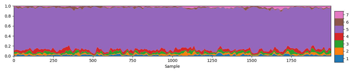
Plotting the raw values of the mixing coefficients as provided by DyNeMo it gives the impression that one mode dominates, in this case mode 4. However, the model DyNeMo uses is \(C_t = \displaystyle\sum_j \alpha_{jt} D_j\), where \(\alpha_{jt}\) are the mixing coefficients and \(D_j\) are the mode covariances. This means a mode can have a small \(\alpha_{jt}\) value but still be a large contributor to the time-varying covariance \(C_t\).

Normalizing the mixing coefficients

To account for the difference in mode covariances we can renormalise the mixing coefficients include the ‘size’ of the mode covariances.

import numpy as np
from osl_dynamics.inference import modes

# Load the inferred mode covariances
covs = np.load("results/inf_params/covs.npy")

# Renormalize the mixing coefficients
norm_alpha = modes.reweight_alphas(alpha, covs)

# Plot the renormalized mixing coefficient time course for the first subject (8 seconds)
fig, ax = plotting.plot_alpha(norm_alpha[0], n_samples=2000)

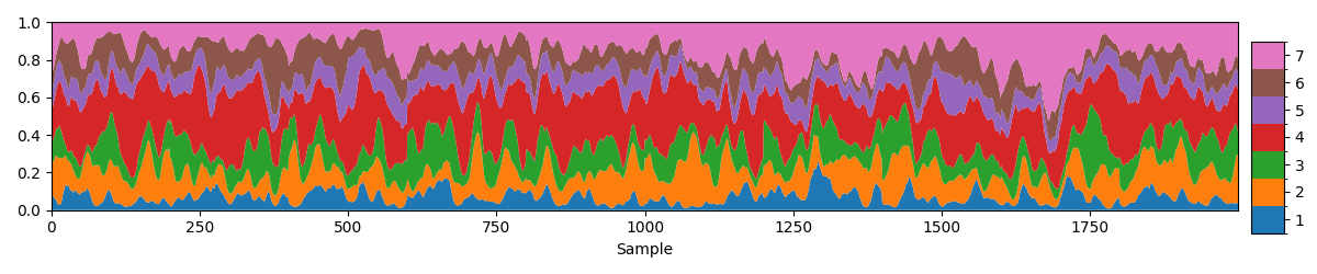
We can now see each mode has a roughly equal contribution to the total covariance. We can also see fast fluctuations in the relative contribution of each mode.

Summary Statistics

An analogous summary measure to the Hidden Markov Model’s (HMM’s) fractional occupancy is the time average mixing coefficient. This is the average contribution a mode makes to the total covariance. Let’s calculate this for each subject.

mean_norm_alpha = np.array([np.mean(a, axis=0) for a in norm_alpha])

# Print group average
print(np.mean(mean_norm_alpha, axis=0))

# Plot distribution over subjects
fig, ax = plotting.plot_violin(mean_norm_alpha.T, x_label="Mode", y_label="Mean alpha")

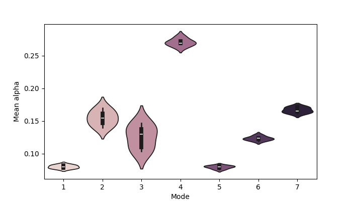
[0.08012532 0.154482   0.12553507 0.27031273 0.07950173 0.1233431
 0.16669996]

Note, we can calculate this using the raw mixing coefficients or the normalized mixing coefficients. We see there is a lot of variability between subjects in terms of this metric.

Another summary measure we could calculate for each subject is the standard deviation of the mixing coefficient time course, which can be a measure for how variable the mixing of each modes is.

std_norm_alpha = np.array([np.std(a, axis=0) for a in norm_alpha])

# Print group average
print(np.mean(std_norm_alpha, axis=0))

# Plot distribution over subjects
fig, ax = plotting.plot_violin(std_norm_alpha.T, x_label="Mode", y_label="Std alpha")

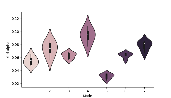
[0.05494202 0.0734943  0.06309029 0.0938042  0.03117273 0.06350952
 0.0783511 ]

Another summary statistic is the kurtosis, which reflects spiking the in mixing coefficient time course.

from scipy import stats

kurt_norm_alpha = np.array([stats.kurtosis(a, axis=0) for a in norm_alpha])

# Print group average
print(np.mean(kurt_norm_alpha, axis=0))

# Plot distribution over subjects
fig, ax = plotting.plot_violin(kurt_norm_alpha.T, x_label="Mode", y_label="Kurt. alpha")

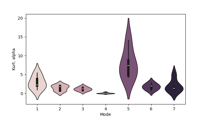
[2.8942084  1.4487444  1.1485741  0.04428925 7.8716993  1.7537019
 1.9642332 ]

Binarizing the mixing coefficient time course

If we convert the mixing coefficients into a binary time course for each mode (i.e. something similar to the HMM state time courses) we can calculate the usual summary statistics we did for the HMM states (fractional occupancies, lifetimes, intervals). See the HMM Summary Statistics tutorial for further details.

We have a couple options for binarizing the mixing coefficient time course:

1. Take the mode with the largest value as ‘on’ while the other modes are ‘off’. This gives a mutually exclusive mode activation time course.

2. Specify a threshold for mode activations. This can be a hand specified threshold or one determined using a data driven approach, such as fitting a Gaussian Mixture Model (GMM). In this case we can have co-activating modes.

Let’s have a look at each of these options.

Binarize with argmax

We can use the inference.modes.argmax_time_courses function to calculate a mutually exclusive mode activation time course.

from osl_dynamics.inference import modes

# Use the mode with the largest value to define mode activations
atc = modes.argmax_time_courses(norm_alpha)

# Plot the mode activation time course for the first subject (first 8 seconds)
fig, ax = plotting.plot_alpha(atc[0], n_samples=2000)

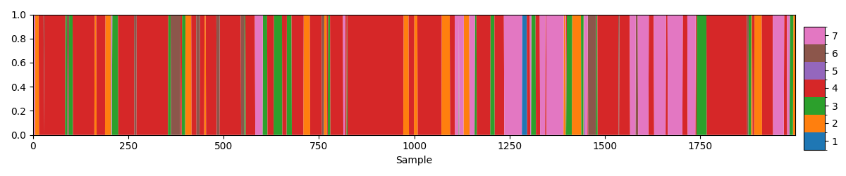
With the mode activation time course we can calculate the usual HMM summary statistics like fractional occupancy.

fo = modes.fractional_occupancies(atc)

# Print group average
print(np.round(np.mean(fo, axis=0), 2))

[0.02 0.11 0.06 0.6  0.   0.05 0.15]

We see there is more of an imbalance between mode activations compared to the HMM state description.

Binarize with a percentile threshold

Next, let’s first specify a threshold by hand. Looking at the distribution of mixing coefficients could help us evaluate a good threshold.

import matplotlib.pyplot as plt

def plot_hist(alpha, x_label=None):
    fig, ax = plt.subplots()
    for i in range(alpha.shape[1]):
        ax.hist(alpha[:, i], label=f"Mode {i+1}", bins=50, histtype="step")
    ax.legend()
    ax.set_xlabel(x_label)

# Concatenate the alphas for each subject
concat_norm_alpha = np.concatenate(norm_alpha)

# Plot their distribution
plot_hist(concat_norm_alpha, x_label="Normalized mixing coefficients")

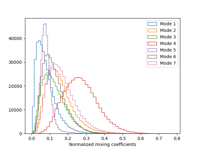
We see the distribution of each mode’s mixing coefficients has a long tail. We’re interested in picking out the time points when the mixing coefficients take values in the long tail. We also see the appropriate threshold for each mode is very different. Let’s use the 90th percentile to determine the threshold of each mode.

thres = np.array([np.percentile(a, 90, axis=0) for a in norm_alpha])

We see the threshold varies a lot across the subjects. Now we have the threshold, let’s binarize.

# Binarize the mixing coefficients
thres_norm_alpha = []
n_subjects = len(norm_alpha)
for na, t in zip(norm_alpha, thres):
    tna = (na > t).astype(int)
    thres_norm_alpha.append(tna)

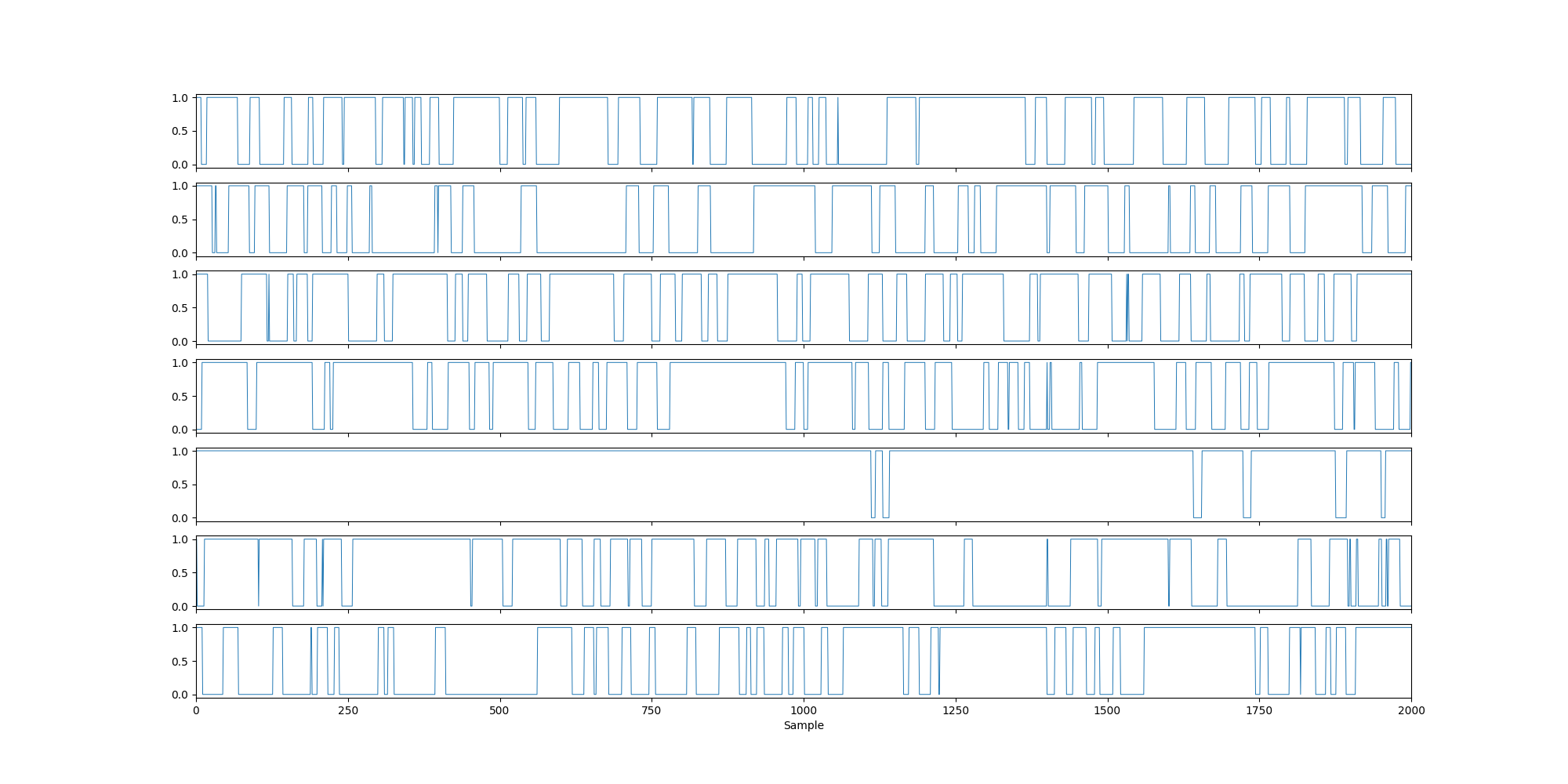
# Plot the mode activation time courses for the first subject (first 8 seconds)
fig, ax = plotting.plot_separate_time_series(thres_norm_alpha[0], n_samples=2000)

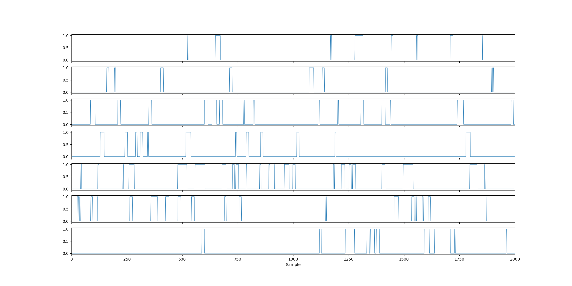
When we threshold using a percentile with the group concatenated data, by definition the fractional occupancy equals the percentile.

fo = modes.fractional_occupancies(thres_norm_alpha)

# Print group average
print(np.mean(fo, axis=0))

[0.1 0.1 0.1 0.1 0.1 0.1 0.1]

We see the fractional occupancy for each subject and state is 0.1, which corresponds to the segments with normalised alpha values in the top 10%. In contrast, the lifetimes are interpretable.

mlt = modes.mean_lifetimes(thres_norm_alpha, sampling_frequency=250)

# Print group average
print(np.mean(mlt, axis=0) * 1000)  # in ms

[57.99183765 63.96468969 50.31304895 58.06805169 76.01930424 50.89961496
 63.0871057 ]

We see with a 90th percentile threshold we get lifetimes of around ~50 ms.

Binarize with a GMM threshold

An aternative approach is to use a two-component GMM to identify an on and off component. This involves fitting the two-component GMM to the distribution of mixing coefficients. We can do this with the inference.modes.gmm_time_courses function in osl-dynamics.

# Binarize the mixing coefficients using a GMM
thres_norm_alpha = modes.gmm_time_courses(norm_alpha)

# Plot the mode activation time courses for the first subject (first 8 seconds)
plotting.plot_separate_time_series(thres_norm_alpha[0], n_samples=2000)

# Display the group average
fo = modes.fractional_occupancies(thres_norm_alpha)
print(np.mean(fo, axis=0), 2)

Fitting GMMs:   0%|          | 0/5 [00:00<?, ?it/s]
Fitting GMMs:  20%|██        | 1/5 [00:02<00:09,  2.34s/it]
Fitting GMMs:  40%|████      | 2/5 [00:04<00:07,  2.37s/it]
Fitting GMMs:  60%|██████    | 3/5 [00:06<00:04,  2.25s/it]
Fitting GMMs:  80%|████████  | 4/5 [00:09<00:02,  2.23s/it]
Fitting GMMs: 100%|██████████| 5/5 [00:11<00:00,  2.28s/it]
Fitting GMMs: 100%|██████████| 5/5 [00:11<00:00,  2.28s/it]
[0.61829376 0.55110528 0.5909216  0.62055283 0.55300455 0.57400481
 0.55981773] 2

We can see the GMM thresholds identify more mode activations, which are reflected in the higher fractional occupancies.

With a mode activation time course we can do the same analysis we did for the HMM state time courses. See the HMM Summary Statistics tutorial for more details.