DyNeMo: Plotting Networks

In this tutorial we will plot networks from a DyNeMo model trained on source reconstructed MEG data. This tutorial covers:

1. Load regression spectra

2. PSDs

3. Power maps

4. Coherence networks

5. Coherence maps

Download post-hoc spectra

In this tutorial, we’ll download example data from OSF.

import os

def get_spectra(name, rename):
    os.system(f"osf -p by2tc fetch spectra/{name}.zip")
    os.makedirs(rename, exist_ok=True)
    os.system(f"unzip -o {name}.zip -d {rename}")
    os.remove(f"{name}.zip")
    return f"Data downloaded to: {rename}"

# Download the dataset (approximately 7 MB)
get_spectra("tde_dynemo_notts_meguk_giles_5_subjects", rename="results/spectra")

'Data downloaded to: results/spectra'

Load regression spectra

We calculate the networks based on the regression spectra. Let’s load these.

import numpy as np

f = np.load("results/spectra/f.npy")
psd = np.load("results/spectra/psd.npy")
coh = np.load("results/spectra/coh.npy")
w = np.load("results/spectra/w.npy")

PSDs

We can plot the power spectra to see what oscillations typically occur when a particular state is on. Let’s first print the shape of the multitaper spectra to understand the format of the data.

print(f.shape)
print(psd.shape)

(45,)
(5, 2, 7, 38, 45)

We can see: f is the frequency axis and psd is a (subjects, 2, modes, channels, frequencies) array. The second axis in psd corresponds to the regression coefficients and intercept when we calculated the mode spectra using analysis.spectral.regression_spectra. The intercept term corresponds to the time average (static) spectra and the regression coefficients describe the variation about the average. We’re not interested in the static spectra, so we just want to retain the regression coefficients.

psd_coefs = psd[:, 0]
print(psd_coefs.shape)

(5, 7, 38, 45)

Now let’s plot the group-average PSD for each mode.

from osl_dynamics.utils import plotting

# Average over subjects and channels
psd_coefs_mean = np.mean(psd_coefs, axis=(0,2))
print(psd_coefs_mean.shape)

# Plot
n_modes = psd_coefs_mean.shape[0]
fig, ax = plotting.plot_line(
    [f] * n_modes,
    psd_coefs_mean,
    labels=[f"Mode {i}" for i in range(1, n_modes + 1)],
    x_label="Frequency (Hz)",
    y_label="PSD (a.u.)",
    x_range=[f[0], f[-1]],
)

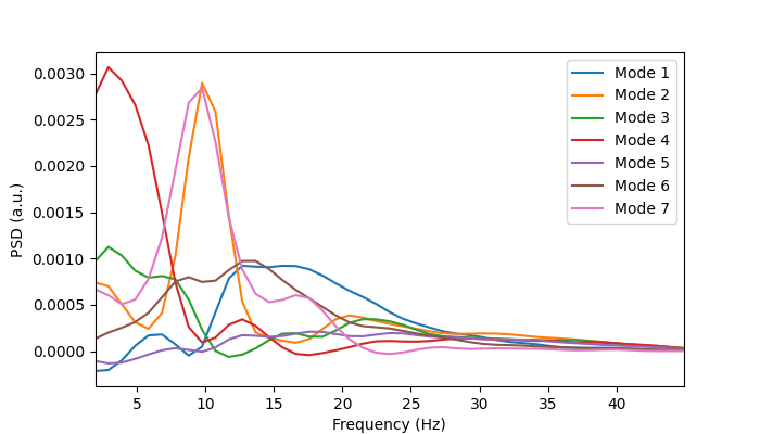
(7, 45)

Power maps

Now let’s integrate the power spectra to calculate the power.

from osl_dynamics.analysis import power

p = power.variance_from_spectra(f, psd_coefs)
print(p.shape)

(5, 7, 38)

We can see p is a (subjects, modes, channels) array. Let’s average over subjects.

mean_p = np.average(p, axis=0, weights=w)
print(mean_p.shape)

(7, 38)

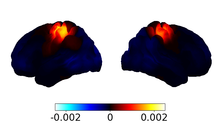
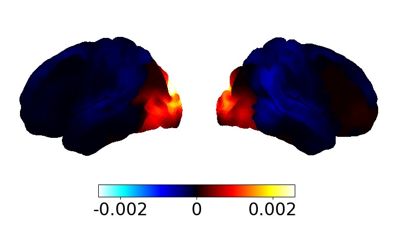
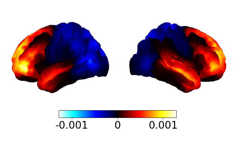
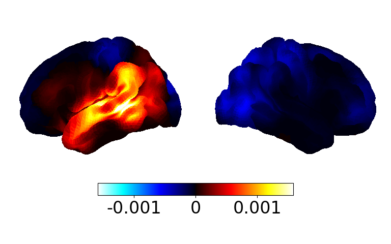
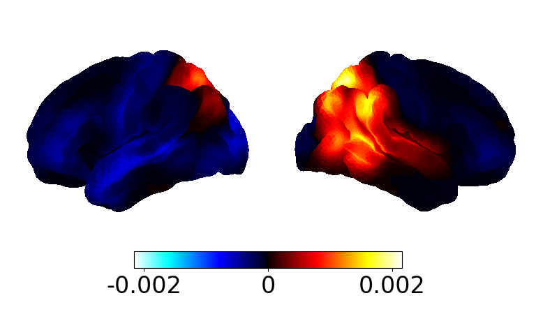
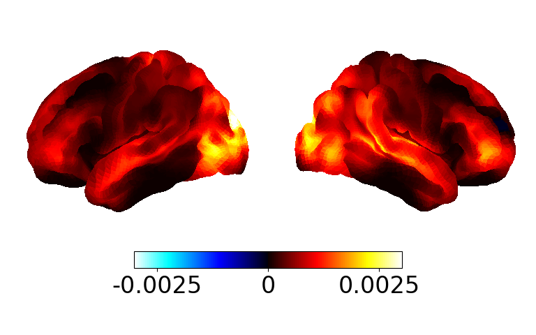
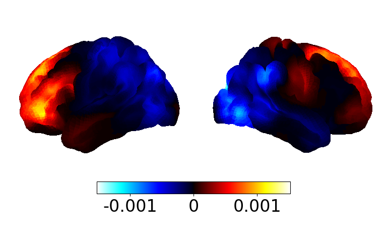
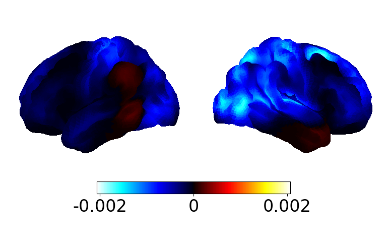
Now we can plot the power map for each mode.

# Display the power maps (takes a few seconds to appear)
fig, ax = power.save(
    mean_p,
    mask_file="MNI152_T1_8mm_brain.nii.gz",
    parcellation_file="atlas-Giles_nparc-38_space-MNI_res-8x8x8.nii.gz",
    subtract_mean=True,  # just for visualisation
)

• 
• 
• 
• 
• 
• 
• 

Saving images:   0%|          | 0/7 [00:00<?, ?it/s]
Saving images:  14%|█▍        | 1/7 [00:00<00:03,  1.88it/s]
Saving images:  29%|██▊       | 2/7 [00:01<00:02,  1.93it/s]
Saving images:  43%|████▎     | 3/7 [00:01<00:02,  1.94it/s]
Saving images:  57%|█████▋    | 4/7 [00:02<00:01,  1.93it/s]
Saving images:  71%|███████▏  | 5/7 [00:02<00:01,  1.91it/s]
Saving images:  86%|████████▌ | 6/7 [00:03<00:00,  1.90it/s]
Saving images: 100%|██████████| 7/7 [00:03<00:00,  1.88it/s]
Saving images: 100%|██████████| 7/7 [00:03<00:00,  1.90it/s]

We can see recognisable functional networks, which gives us confidence in the DyNeMo fit. We also see the networks are more localised than typical HMM states.

Coherence networks

Next, let’s visualise the coherence networks. First, we need to calculate the networks from the coherence spectra.

print(coh.shape)

(5, 7, 38, 38, 45)

We can see the coherence spectra is a (subjects, modes, channels, channels, frequencies) array. Let’s calculate the mean coherence over all frequencies.

from osl_dynamics.analysis import connectivity

c = connectivity.mean_coherence_from_spectra(f, coh)
print(c.shape)

(5, 7, 38, 38)

We now have a (subjects, modes, channels, channels) array. Next we need to average over subjects and threshold the coherence networks.

# Average over subjects
mean_c = np.average(c, axis=0, weights=w)

# Threshold the top 3% relative to the mean
thres_mean_c = connectivity.threshold(mean_c, percentile=97, subtract_mean=True)

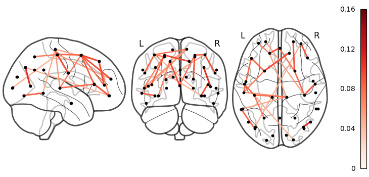
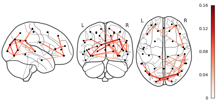
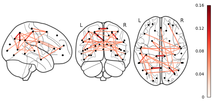
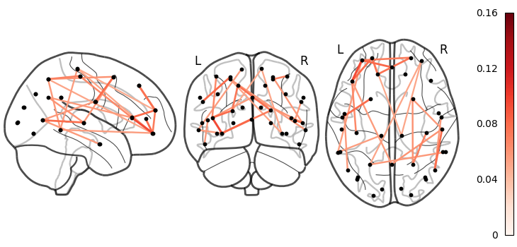
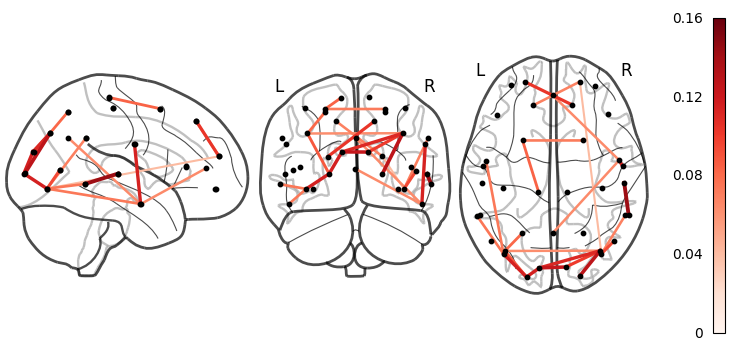
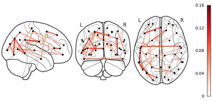
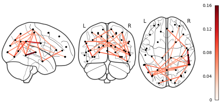
Now we can visualise the networks.

connectivity.save(
    thres_mean_c,
    parcellation_file="atlas-Giles_nparc-38_space-MNI_res-8x8x8.nii.gz",
    plot_kwargs={"edge_vmin": 0, "edge_vmax": np.max(thres_mean_c), "edge_cmap": "Reds"},
)

• 
• 
• 
• 
• 
• 
• 

Saving images:   0%|          | 0/7 [00:00<?, ?it/s]
Saving images:  14%|█▍        | 1/7 [00:00<00:03,  1.85it/s]
Saving images:  29%|██▊       | 2/7 [00:01<00:02,  1.87it/s]
Saving images:  43%|████▎     | 3/7 [00:01<00:02,  1.87it/s]
Saving images:  57%|█████▋    | 4/7 [00:02<00:01,  1.86it/s]
Saving images:  71%|███████▏  | 5/7 [00:03<00:01,  1.41it/s]
Saving images:  86%|████████▌ | 6/7 [00:03<00:00,  1.54it/s]
Saving images: 100%|██████████| 7/7 [00:04<00:00,  1.65it/s]
Saving images: 100%|██████████| 7/7 [00:04<00:00,  1.66it/s]

We can see the coherence networks show high coherence in the same regions with high power. We expect these networks will improve with more subjects.

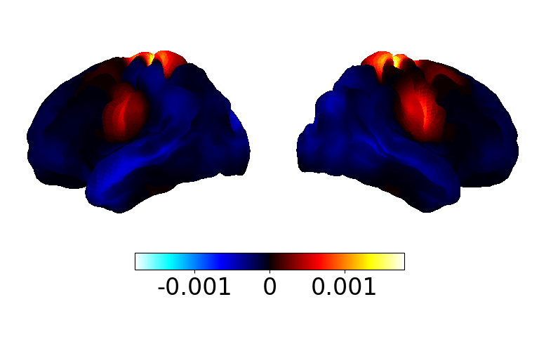
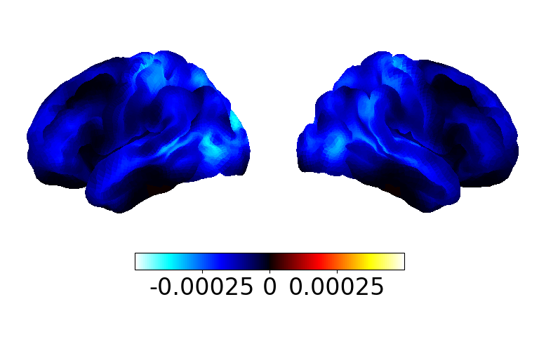
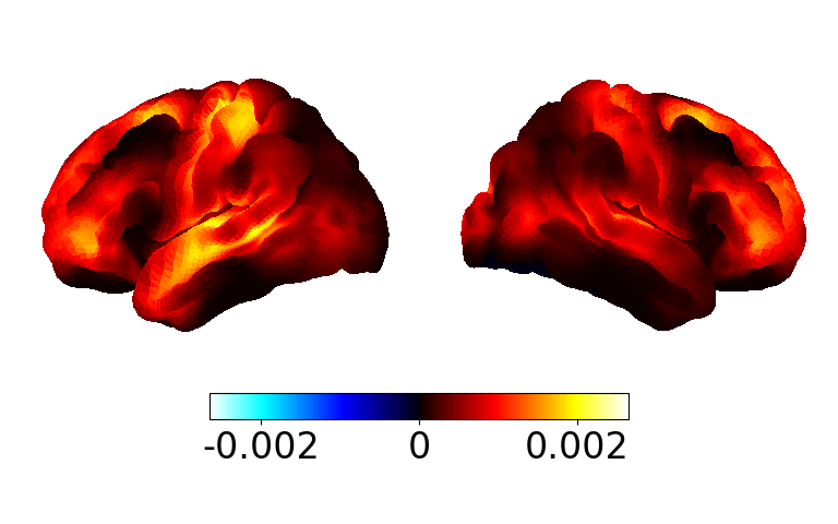
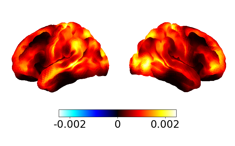
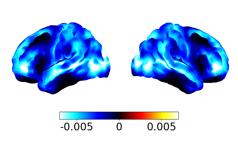
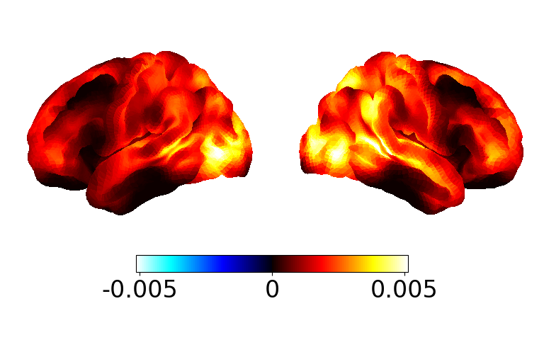
Coherence maps

We can display the coherence as a spatial map rather than a graphical network by averaging the edges for each parcel.

mean_c_map = connectivity.mean_connections(mean_c)

fig, ax = power.save(
    mean_c_map,
    mask_file="MNI152_T1_8mm_brain.nii.gz",
    parcellation_file="atlas-Giles_nparc-38_space-MNI_res-8x8x8.nii.gz",
    subtract_mean=True,  # just for visualisation
)

• 
• 
• 
• 
• 
• 
• 

Saving images:   0%|          | 0/7 [00:00<?, ?it/s]
Saving images:  14%|█▍        | 1/7 [00:01<00:06,  1.06s/it]
Saving images:  29%|██▊       | 2/7 [00:01<00:04,  1.24it/s]
Saving images:  43%|████▎     | 3/7 [00:02<00:02,  1.37it/s]
Saving images:  57%|█████▋    | 4/7 [00:02<00:02,  1.43it/s]
Saving images:  71%|███████▏  | 5/7 [00:03<00:01,  1.47it/s]
Saving images:  86%|████████▌ | 6/7 [00:04<00:00,  1.48it/s]
Saving images: 100%|██████████| 7/7 [00:04<00:00,  1.48it/s]
Saving images: 100%|██████████| 7/7 [00:04<00:00,  1.41it/s]