HMM: Summary Statistics

A useful way of characterising the data is to use statistics that summarise the state time course, these are referred to as ‘summary statistics’. The state time course captures the dynamics in the training data, therefore, summary statistics characterise the dynamics of the data.

In this tutorial we calculate summary statistics for dynamics:

• Fractional occupancy, which is the fraction of total time spent in a particular state.

• Mean lifetime, which is the average duration a state is activate.

• Mean interval, which is the average duration between successive state visits.

• Switching rate, which is the average number of state activations.

Download inferred parameters

import os

def get_inf_params(name, rename):
    os.system(f"osf -p by2tc fetch inf_params/{name}.zip")
    os.makedirs(rename, exist_ok=True)
    os.system(f"unzip -o {name}.zip -d {rename}")
    os.remove(f"{name}.zip")
    return f"Data downloaded to: {rename}"

# Download the dataset (approximately 11 MB)
get_inf_params("tde_hmm_notts_meguk_giles_5_subjects", rename="results/inf_params")

'Data downloaded to: results/inf_params'

Load the inferred state probabilities

We first need to load the inferred state probabilities to calculate the summary statistics.

import pickle

alpha = pickle.load(open("results/inf_params/alp.pkl", "rb"))

Let’s also plot the state probabilities for the first few seconds of the first subject to get a feel for what they look like. We can use the utils.plotting.plot_alpha function to do this.

from osl_dynamics.utils import plotting

# Plot the state probability time course for the first subject (8 seconds)
fig, ax = plotting.plot_alpha(alpha[0], n_samples=2000)

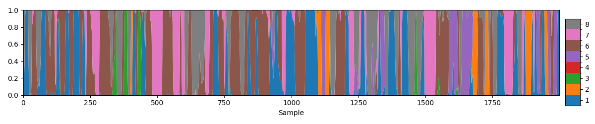
When looking at the state probability time course you want to see a good number of transitions between states.

The alpha list contains the state probabilities time course for each subject. To calculate summary statistics we first need to hard classify the state probabilities to give a state time course. We can use the inference.modes.argmax_time_courses function to do this.

from osl_dynamics.inference import modes

# Hard classify the state probabilities
stc = modes.argmax_time_courses(alpha)

# Plot the state time course for the first subject (8 seconds)
fig, ax = plotting.plot_alpha(stc[0], n_samples=2000)

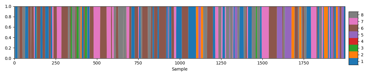
We can see this time series is completely binarised, only one state is active at each time point.

Calculate summary statistics

Fractional occupancy

The analysis.post_hoc module in osl-dynamics contains helpful functions for calculating summary statistics. Let’s use the analysis.post_hoc.fractional_occupancies function to calculate the fractional occupancy of each state for each subject.

from osl_dynamics.analysis import post_hoc

# Calculate fractional occupancies
fo = post_hoc.fractional_occupancies(stc)
print(fo.shape)

(5, 8)

We can see fo is a (subjects, states) numpy array which contains the fractional occupancy of each state for each subject.

To get a feel for how much each state is activated we can print the group average:

import numpy as np

print(np.mean(fo, axis=0))

[0.17031502 0.10770698 0.136075   0.03785646 0.15199955 0.16724242
 0.06957335 0.15923123]

We can see each state shows a significant activation (i.e. non-zero), which gives us confidence in the fit. If only one state is activated, that indicates further preprocessing is likely needed.

We can examine the distribution across subjects for each state by creating a violin plot. The utils.plotting.plot_violin function can be used to do this.

# Plot the distribution of fractional occupancy (FO) across subjects
fig, ax = plotting.plot_violin(fo.T, x_label="State", y_label="Fractional Occupancy")

We can see there is a lot of variation across subjects.

Mean Lifetime

Next, let’s look at another popular summary statistic, i.e. the mean lifetime. We can calculate this using the analysis.post_hoc.mean_lifetimes function.

# Calculate mean lifetimes (in seconds)
lt = post_hoc.mean_lifetimes(stc, sampling_frequency=250)

# Convert to ms
lt *= 1000

# Print the group average
print(np.mean(lt, axis=0))

# Plot distribution across subjects
fig, ax = plotting.plot_violin(lt.T, x_label="State", y_label="Mean Lifetime (ms)")

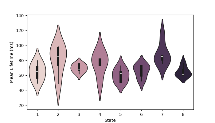
[64.5703925  80.69838401 69.58749073 75.8973731  60.17574585 65.52617621
 88.21728058 64.86945622]

Mean interval

Next, let’s look at the mean interval time for each state and subject. We can use the analysis.post_hoc.mean_intervals function in osl-dynamics to calculate this.

# Calculate mean intervals (in seconds)
intv = post_hoc.mean_intervals(stc, sampling_frequency=250)

# Print the group average
print(np.mean(intv, axis=0))

# Plot distribution across subjects
fig, ax = plotting.plot_violin(intv.T, x_label="State", y_label="Mean Interval (s)")

[0.32125534 0.7271179  0.45446391 2.32690234 0.38967127 0.33346291
 1.44239173 0.35297459]

Switching rate

Finally, let’s look at the switching rate for each state and subject. We can use the analysis.post_hoc.switching_rate function in osl-dynamics to calculate this.

# Calculate the switching rate (Hz)
sr = post_hoc.switching_rates(stc, sampling_frequency=250)

# Print the group average
print(np.mean(sr, axis=0))

# Plot distribution across subjects
fig, ax = plotting.plot_violin(sr.T, x_label="State", y_label="Switching Rate (Hz)")

[2.60825826 1.30724474 1.97700826 0.47477477 2.42391141 2.54483859
 0.8201952  2.48825075]