Note

Go to the end to download the full example code.

HMM: Plotting MEG Networks#

In this tutorial we will plot networks from an HMM trained on source reconstructed MEG data. This tutorial covers:

Load multitaper spectra
PSDs
Power maps
Coherence networks
Coherence maps
Coherence vs Power

Download post-hoc spectra#

In this tutorial, we’ll download example data from OSF.

import os

def get_spectra(name, rename):
    os.system(f"osf -p by2tc fetch spectra/{name}.zip")
    os.makedirs(rename, exist_ok=True)
    os.system(f"unzip -o {name}.zip -d {rename}")
    os.remove(f"{name}.zip")
    return f"Data downloaded to: {rename}"

# Download the dataset (approximately 21 MB)
get_spectra("tde_hmm_notts_meguk_giles_5_subjects", rename="results/spectra")

'Data downloaded to: results/spectra'

Load multitaper spectra#

We calculate networks based on multitaper spectra. Let’s load these.

import numpy as np

f = np.load("results/spectra/f.npy")
psd = np.load("results/spectra/psd.npy")
coh = np.load("results/spectra/coh.npy")
w = np.load("results/spectra/w.npy")

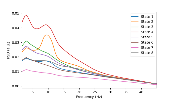
PSDs#

We can plot the power spectra to see what oscillations typically occur when a particular state is on. Let’s first print the shape of the multitaper spectra to understand the format of the data.

print(f.shape)
print(psd.shape)

(90,)
(5, 8, 38, 90)

From the shape of each array we can see f is a 1D numpy array which contains the frequency axis of the spectra and psd is a (subjects, states, channels, frequencies) array.

To help us visualise this we can average over the subjects and channels. This gives us a (states, frequencies) array.

from osl_dynamics.utils import plotting

# Average over subjects and channels
gpsd = np.average(psd, axis=0, weights=w)
psd_mean = np.mean(gpsd, axis=1)
print(psd_mean.shape)

# Plot
n_states = psd_mean.shape[0]
fig, ax = plotting.plot_line(
    [f] * n_states,
    psd_mean,
    labels=[f"State {i}" for i in range(1, n_states + 1)],
    x_label="Frequency (Hz)",
    y_label="PSD (a.u.)",
    x_range=[f[0], f[-1]],
)

(8, 90)

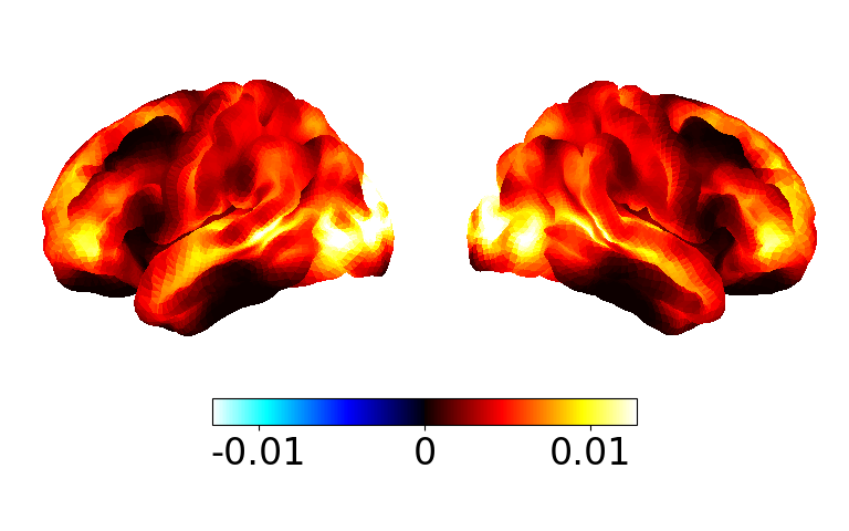
Power maps#

The psd array contains the spectrum for each channel (for each subject/state). This is a function of frequency. To calculate power we need to integrate over a frequency range. osl-dynamics has the analysis.power.variance_from_spectra function to help us do this. Let’s look at the power across all frequencies for a given state.

from osl_dynamics.analysis import power

p = power.variance_from_spectra(f, psd)
print(p.shape)

(5, 8, 38)

We have a power map for each state and subject. Let’s calculate the group average.

p_mean = np.average(p, axis=0, weights=w)
print(p_mean.shape)

(8, 38)

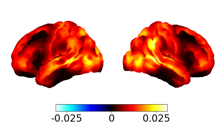
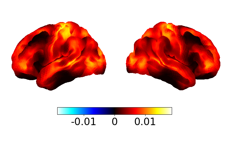
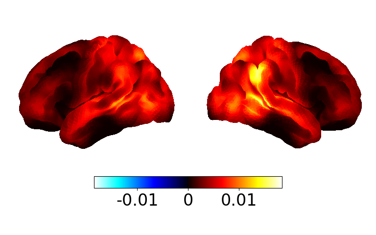
Now we have a (states, channels) array. Let’s see what the power map for each state looks like.

# Takes a few seconds for the power maps to appear
fig, ax = power.save(
    p_mean,
    mask_file="MNI152_T1_8mm_brain.nii.gz",
    parcellation_file="atlas-Giles_nparc-38_space-MNI_res-8x8x8.nii.gz",
)

Saving images:   0%|          | 0/8 [00:00<?, ?it/s]
Saving images:  12%|█▎        | 1/8 [00:00<00:03,  1.97it/s]
Saving images:  25%|██▌       | 2/8 [00:01<00:03,  1.96it/s]
Saving images:  38%|███▊      | 3/8 [00:01<00:02,  1.96it/s]
Saving images:  50%|█████     | 4/8 [00:02<00:02,  1.97it/s]
Saving images:  62%|██████▎   | 5/8 [00:02<00:01,  1.97it/s]
Saving images:  75%|███████▌  | 6/8 [00:03<00:01,  1.94it/s]
Saving images:  88%|████████▊ | 7/8 [00:03<00:00,  1.92it/s]
Saving images: 100%|██████████| 8/8 [00:04<00:00,  1.91it/s]
Saving images: 100%|██████████| 8/8 [00:04<00:00,  1.94it/s]

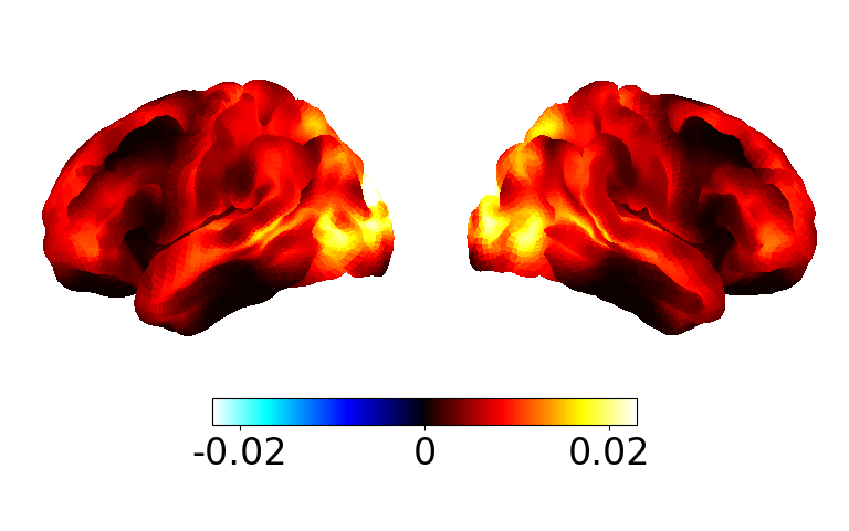
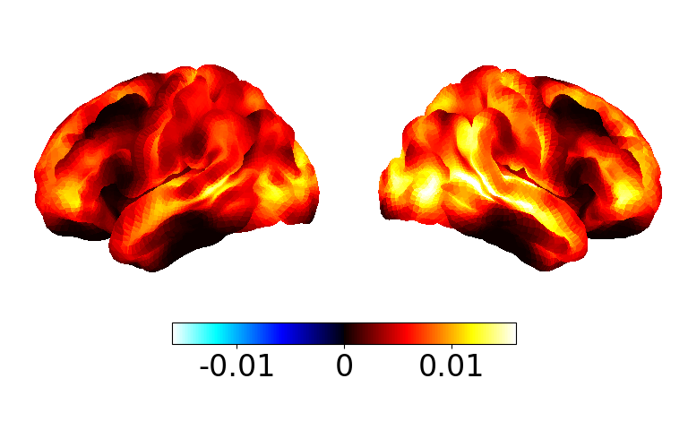
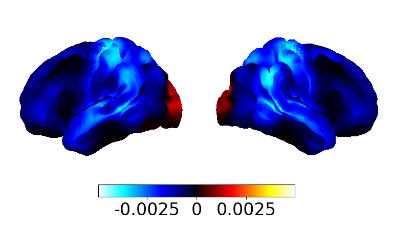
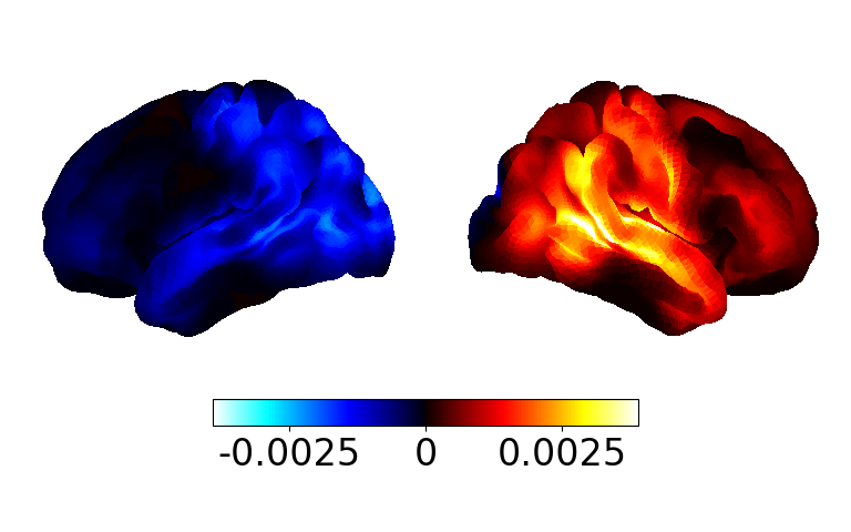
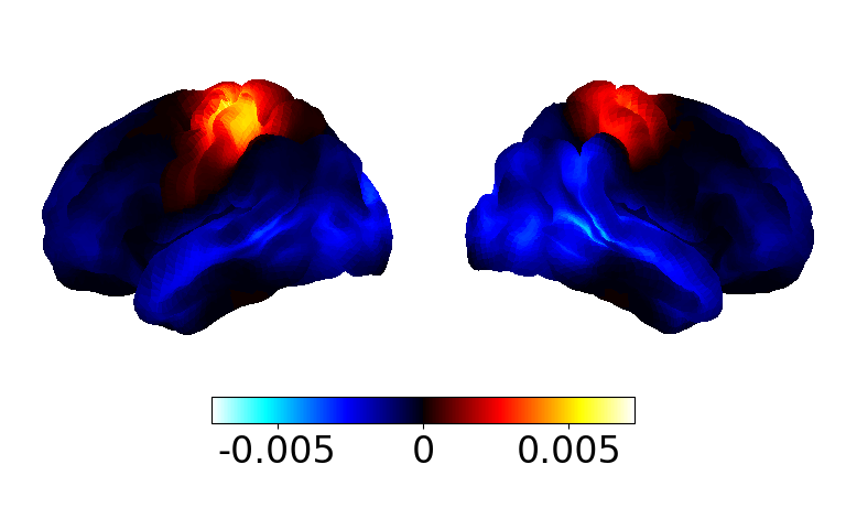
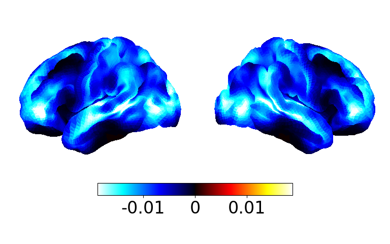
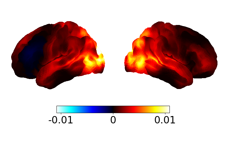
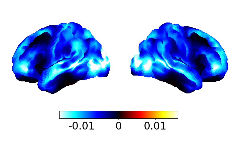
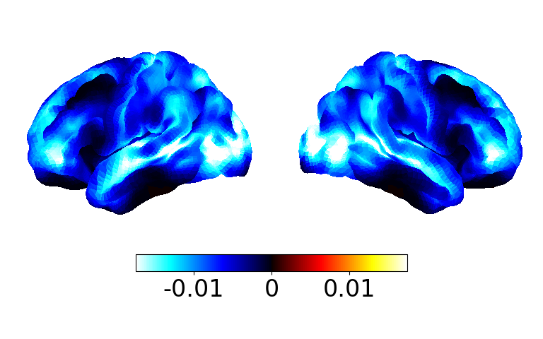
Because the power is always positive and a lot of the state have power in similar regions all the power maps look similar. To highlight differences we can display the power maps relative to something. Typically we use the average across states - taking the average across states approximates the static power of the entire training dataset. We can do this by passing the subtract_mean argument.

# Takes a few seconds for the power maps to appear
fig, ax = power.save(
    p_mean,
    mask_file="MNI152_T1_8mm_brain.nii.gz",
    parcellation_file="atlas-Giles_nparc-38_space-MNI_res-8x8x8.nii.gz",
    subtract_mean=True,
)

Saving images:   0%|          | 0/8 [00:00<?, ?it/s]
Saving images:  12%|█▎        | 1/8 [00:00<00:04,  1.68it/s]
Saving images:  25%|██▌       | 2/8 [00:01<00:03,  1.67it/s]
Saving images:  38%|███▊      | 3/8 [00:01<00:03,  1.66it/s]
Saving images:  50%|█████     | 4/8 [00:02<00:02,  1.65it/s]
Saving images:  62%|██████▎   | 5/8 [00:03<00:01,  1.62it/s]
Saving images:  75%|███████▌  | 6/8 [00:03<00:01,  1.60it/s]
Saving images:  88%|████████▊ | 7/8 [00:04<00:00,  1.60it/s]
Saving images: 100%|██████████| 8/8 [00:04<00:00,  1.58it/s]
Saving images: 100%|██████████| 8/8 [00:04<00:00,  1.61it/s]

Coherence networks#

Next, let’s visualise the coherence networks. First, we need to calculate the networks from the coherence spectra.

print(coh.shape)

(5, 8, 38, 38, 90)

We can see coh is a (subjects, states, channels, channels, frequencies) array. Let’s calculate the mean coherence over all frequencies.

from osl_dynamics.analysis import connectivity

c = connectivity.mean_coherence_from_spectra(f, coh)
print(c.shape)

(5, 8, 38, 38)

Note, if we were interested in a particular frequency band we could use the frequency_range argument to specify the range.

We can see from the shape of c it is a (subjects, states, channels, channels) array. The c[0][0] element corresponds to the (n_channels, n_channels) coherence network for the first subject and state.

Coherence networks are often noisy so averaging over a large number of subjects (20+) is typically needed to get clean coherence networks. Let’s average the coherence networks over all subjects.

mean_c = np.average(c, axis=0, weights=w)
print(mean_c.shape)

(8, 38, 38)

We now see c_mean is a (states, channels, channels) array.

Let’s have a look at the coherence networks. The connectivity.save function can be used to display a connectivity matrix (or set of connectivity matrices). Note, we display them relative to the mean across states.

mean_c -= np.mean(mean_c, axis=0)
connectivity.save(
    mean_c,
    parcellation_file="atlas-Giles_nparc-38_space-MNI_res-8x8x8.nii.gz",
)

Saving images:   0%|          | 0/8 [00:00<?, ?it/s]
Saving images:  12%|█▎        | 1/8 [00:01<00:11,  1.70s/it]
Saving images:  25%|██▌       | 2/8 [00:03<00:12,  2.04s/it]
Saving images:  38%|███▊      | 3/8 [00:06<00:11,  2.22s/it]
Saving images:  50%|█████     | 4/8 [00:08<00:08,  2.07s/it]
Saving images:  62%|██████▎   | 5/8 [00:10<00:06,  2.21s/it]
Saving images:  75%|███████▌  | 6/8 [00:12<00:04,  2.03s/it]
Saving images:  88%|████████▊ | 7/8 [00:14<00:01,  1.91s/it]
Saving images: 100%|██████████| 8/8 [00:16<00:00,  2.17s/it]
Saving images: 100%|██████████| 8/8 [00:16<00:00,  2.10s/it]

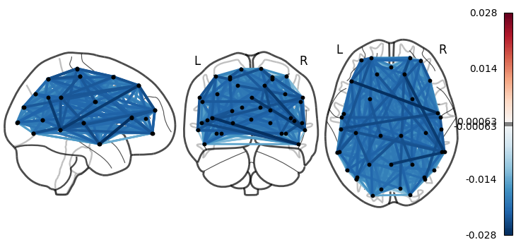
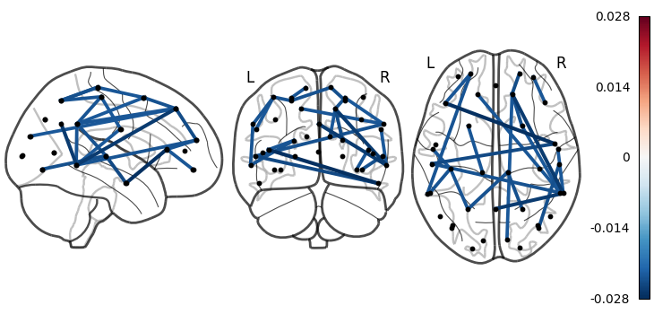
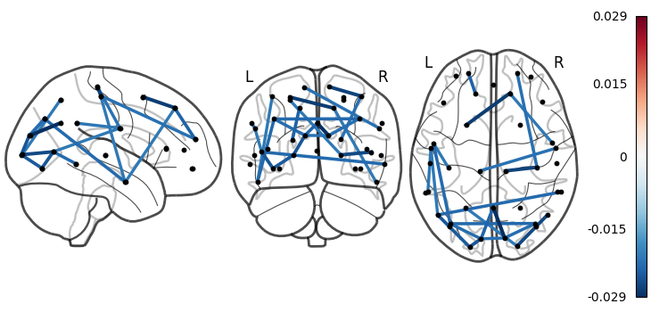
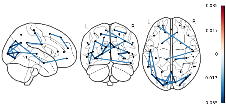
We can see there are a lot of connections. We want to select the most extreme edeges. osl-dynamics has a function called connectivity.threshold that makes this easy.

thres_mean_c = connectivity.threshold(mean_c, percentile=97, absolute_value=True)
print(thres_mean_c.shape)

(8, 38, 38)

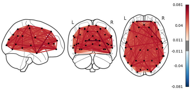
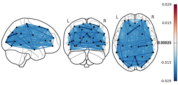
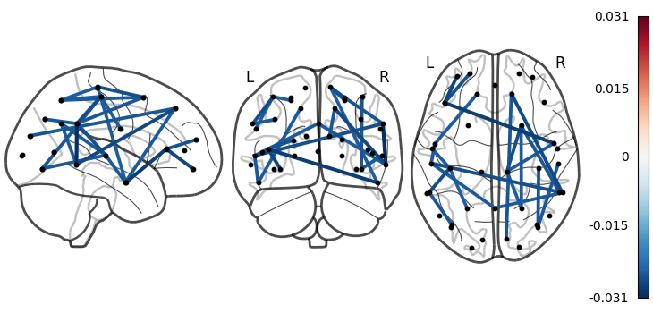
Now let’s visualise the thresholded networks.

connectivity.save(
    thres_mean_c,
    parcellation_file="atlas-Giles_nparc-38_space-MNI_res-8x8x8.nii.gz",
)

Saving images:   0%|          | 0/8 [00:00<?, ?it/s]
Saving images:  12%|█▎        | 1/8 [00:00<00:03,  1.82it/s]
Saving images:  25%|██▌       | 2/8 [00:01<00:03,  1.82it/s]
Saving images:  38%|███▊      | 3/8 [00:01<00:02,  1.83it/s]
Saving images:  50%|█████     | 4/8 [00:02<00:02,  1.84it/s]
Saving images:  62%|██████▎   | 5/8 [00:02<00:01,  1.84it/s]
Saving images:  75%|███████▌  | 6/8 [00:03<00:01,  1.84it/s]
Saving images:  88%|████████▊ | 7/8 [00:03<00:00,  1.84it/s]
Saving images: 100%|██████████| 8/8 [00:04<00:00,  1.83it/s]
Saving images: 100%|██████████| 8/8 [00:04<00:00,  1.83it/s]

Non-negative matrix factorization (NNMF)#

In the above code, we integrated over all frequencies to calculate the power maps and coherence networks. We expect brain activity to occur with phase-locking networks with oscillations at different frequencies. A data-driven approach for finding the frequency bands (referred to as ‘spectral components’) for phase-locked networks is to apply non-negative matrix factorization (NNMF) to the coherence spectra for each subject. osl-dynamics has a function that can do this: analysis.spectral.decompose_spectra. Let’s use this function to separate our coherence spectra (coh) into two frequency bands.

from osl_dynamics.analysis import spectral

# Perform NNMF on the coherence spectra of each subject (we concatenate each matrix)
wb_comp = spectral.decompose_spectra(coh, n_components=2)
print(wb_comp.shape)

(2, 90)

wb_comp refers to ‘wideband component’ because the spectral components cover a wide frequency range (we’ll see this below). If we passed n_components=4, we would find more narrowband components. You can interpret the wb_comp array as weights for how much coherent (phase-locking) activity is occurring at a particular frequency for a particular component. It can be better understood if we plot it.

from osl_dynamics.utils import plotting

plotting.plot_line(
    [f, f],  # we need to repeat twice because we fitted two components
    wb_comp,
    x_label="Frequency (Hz)",
    y_label="Spectral Component",
)

(<Figure size 700x400 with 1 Axes>, <Axes: xlabel='Frequency (Hz)', ylabel='Spectral Component'>)

The blue line is the first spectral component and the orange line is the second component. We can see the NNMF has separated the coherence spectra into two bands, one with a lot of coherence activity below ~22 Hz (blue line) and one above (orange line). In other words, the first spectral component contains coherent activity below 22 Hz and the second contains coherent activity mainly above 22 Hz.

Now, instead of averaging the coherence spectra across all frequencies, let’s just look at the first spectral component (we calculate the coherence network by weighting each frequency in the coherence spectra using the spectral component).

# Calculate the coherence network for each state by weighting with the spectral components
c = connectivity.mean_coherence_from_spectra(f, coh, wb_comp)
print(c.shape)

# Average over subjects
mean_c = np.average(c, axis=0, weights=w)
print(mean_c.shape)

# Threshold each network and look for the top 3% of connections relative to the mean
mean_c -= np.mean(mean_c, axis=1, keepdims=True)  # subtract mean across states
thres_mean_c = connectivity.threshold(mean_c, percentile=97, absolute_value=True)
print(thres_mean_c.shape)

(5, 2, 8, 38, 38)
(2, 8, 38, 38)
(2, 8, 38, 38)

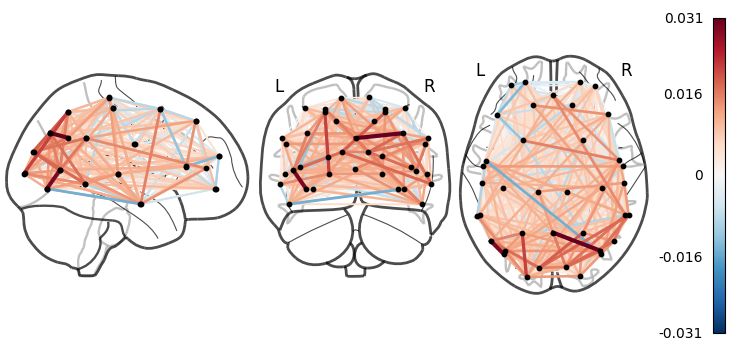
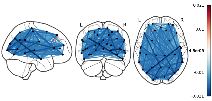
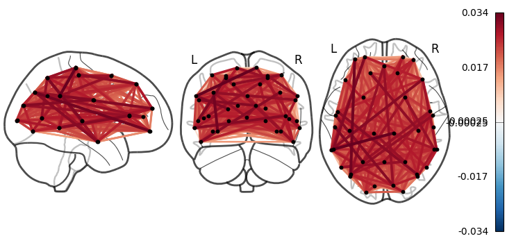
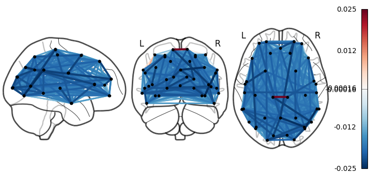
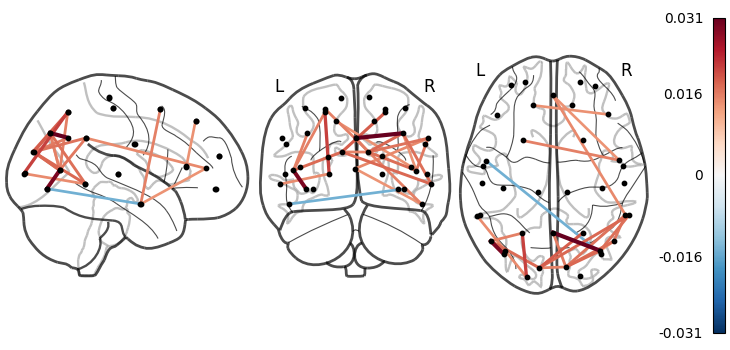
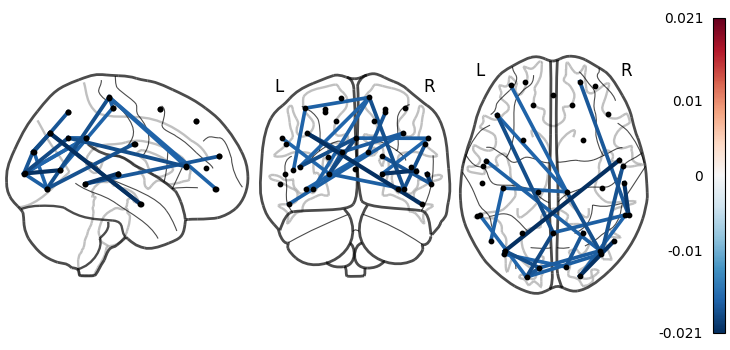
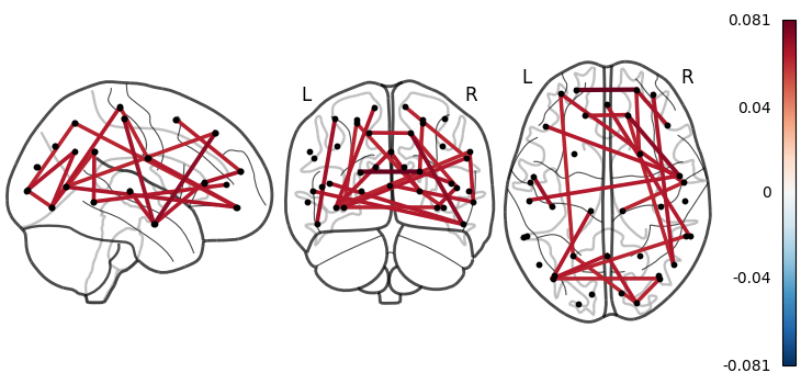
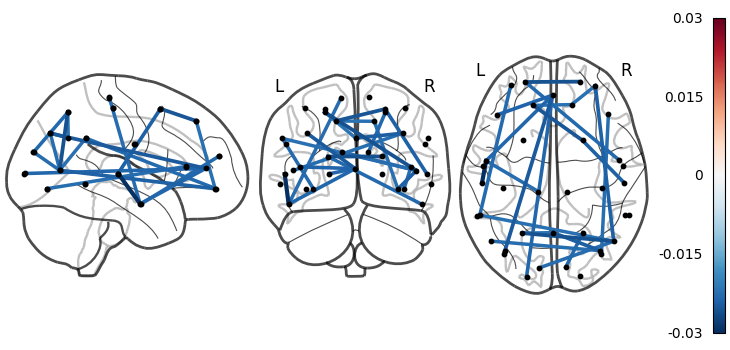
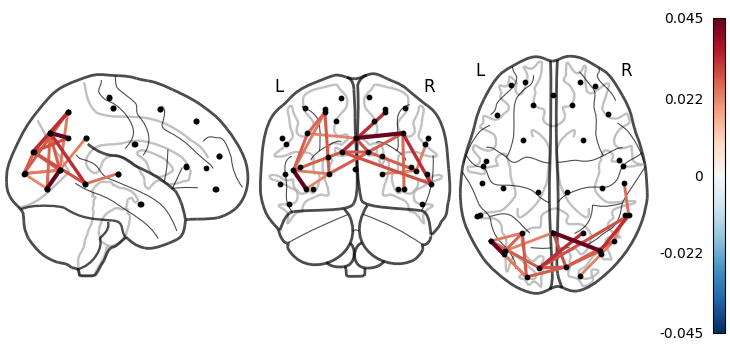
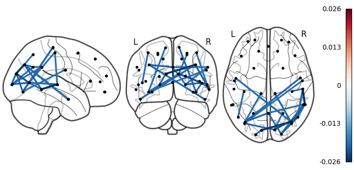
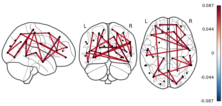
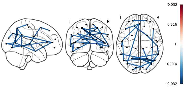
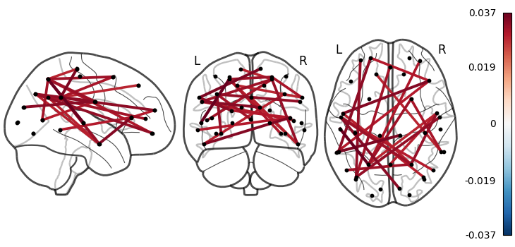
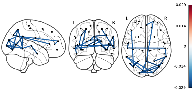
We can see the c_mean and c_mean_thres array here is (components, states, channels, channels). We’re only interested in the first spectral component. We can plot this by passing a component=0 argument to connectivity.save.

connectivity.save(
    thres_mean_c,
    parcellation_file="atlas-Giles_nparc-38_space-MNI_res-8x8x8.nii.gz",
    component=0,
)

Saving images:   0%|          | 0/8 [00:00<?, ?it/s]
Saving images:  12%|█▎        | 1/8 [00:03<00:22,  3.15s/it]
Saving images:  25%|██▌       | 2/8 [00:03<00:09,  1.62s/it]
Saving images:  38%|███▊      | 3/8 [00:04<00:05,  1.13s/it]
Saving images:  50%|█████     | 4/8 [00:04<00:03,  1.11it/s]
Saving images:  62%|██████▎   | 5/8 [00:05<00:02,  1.30it/s]
Saving images:  75%|███████▌  | 6/8 [00:05<00:01,  1.44it/s]
Saving images:  88%|████████▊ | 7/8 [00:06<00:00,  1.21it/s]
Saving images: 100%|██████████| 8/8 [00:07<00:00,  1.36it/s]
Saving images: 100%|██████████| 8/8 [00:07<00:00,  1.06it/s]

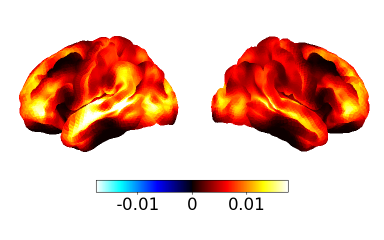
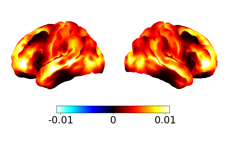
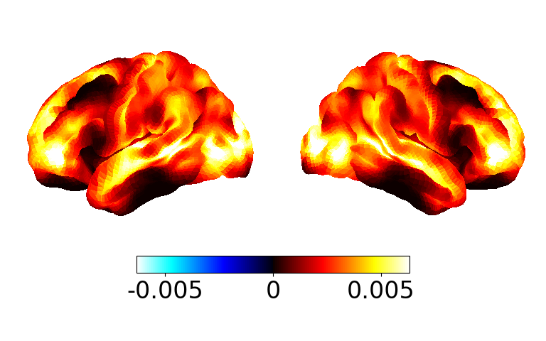
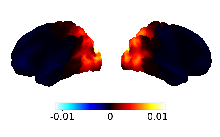
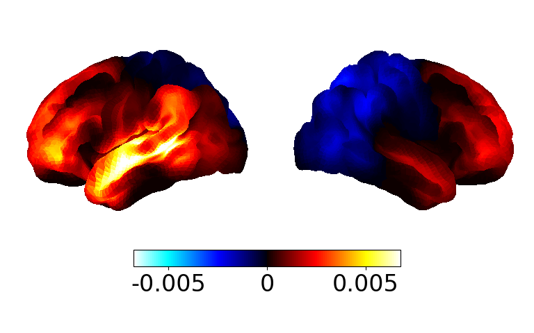
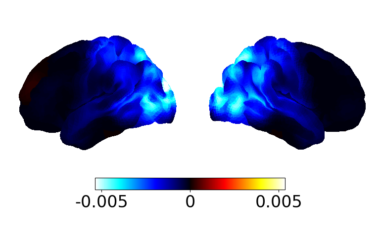
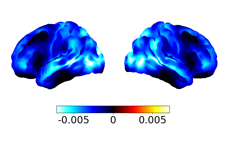
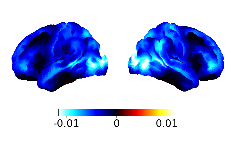
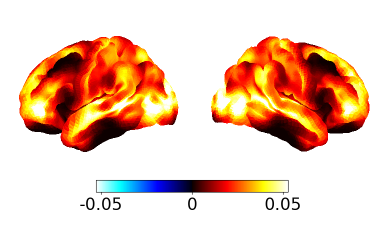
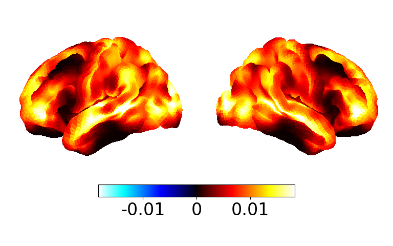
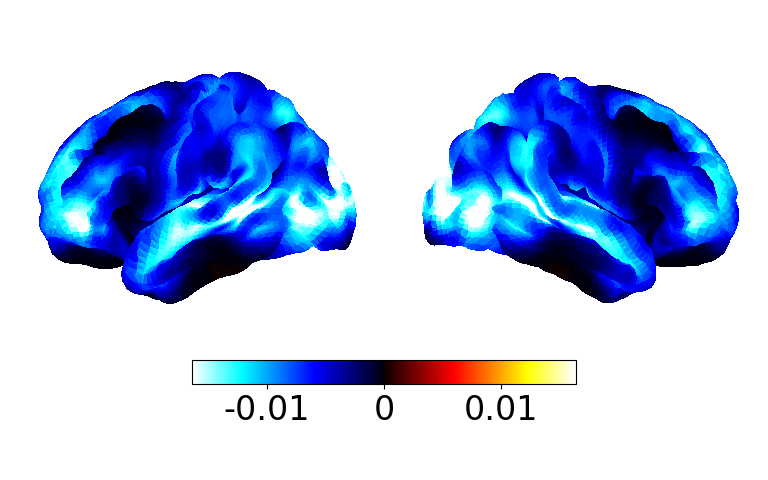
Coherence maps#

We can display the coherence as a spatial map rather than a graphical network by averaging the edges for each parcel.

mean_c_map = connectivity.mean_connections(mean_c)

fig, ax = power.save(
    mean_c_map,
    mask_file="MNI152_T1_8mm_brain.nii.gz",
    parcellation_file="atlas-Giles_nparc-38_space-MNI_res-8x8x8.nii.gz",
)

Saving images:   0%|          | 0/8 [00:00<?, ?it/s]
Saving images:  12%|█▎        | 1/8 [00:01<00:08,  1.21s/it]
Saving images:  25%|██▌       | 2/8 [00:01<00:05,  1.14it/s]
Saving images:  38%|███▊      | 3/8 [00:02<00:03,  1.30it/s]
Saving images:  50%|█████     | 4/8 [00:03<00:02,  1.39it/s]
Saving images:  62%|██████▎   | 5/8 [00:03<00:02,  1.44it/s]
Saving images:  75%|███████▌  | 6/8 [00:04<00:01,  1.45it/s]
Saving images:  88%|████████▊ | 7/8 [00:05<00:00,  1.48it/s]
Saving images: 100%|██████████| 8/8 [00:05<00:00,  1.49it/s]
Saving images: 100%|██████████| 8/8 [00:05<00:00,  1.38it/s]

Coherence vs Power#

We may be interested in how the coherence relates to power for each state. We can do this by producing scatter plots of coherence vs power. Let’s see how to do this.

# Calculate power
p = power.variance_from_spectra(f, psd, wb_comp)
print(p.shape)

# Calculate coherence
c = connectivity.mean_coherence_from_spectra(f, coh, wb_comp)
print(c.shape)

(5, 2, 8, 38)
(5, 2, 8, 38, 38)

Now we want to summarise the power and coherence for each state. We could do this by:

Averaging over subjects to get the power/coherence for each parcel.
Averaging over parcels to get the power/coherence for each subject.

Let’s first average the power and coherence over subjects and select the first spectral component.

# Average power over subjects
mean_p = np.mean(p, axis=0)
print(mean_p.shape)

# Average coherence over subjects
mean_c = np.mean(c, axis=0)
print(mean_c.shape)

# Keep the first spectral component
mean_p = mean_p[0]
mean_c = mean_c[0]
print(mean_p.shape)
print(mean_c.shape)

(2, 8, 38)
(2, 8, 38, 38)
(8, 38)
(8, 38, 38)

We have a (n_channels,) array for each state for the power, but a (n_channels, n_channels) array for each state for the coherence. To reduce the coherence down to a 1D array for each state, we can calculate the average pairwise coherence for each channels. We can do this with the connectivity.mean_connections function.

mean_c = connectivity.mean_connections(mean_c)
print(mean_c.shape)

(8, 38)

Now we can make a scatter plot of coherence vs power for each state.

fig, ax = plotting.plot_scatter(
    mean_p,
    mean_c,
    labels=[f"State {i}" for i in range(1, mean_p.shape[0] + 1)],
    x_label="Power (a.u.)",
    y_label="Coherence",
)

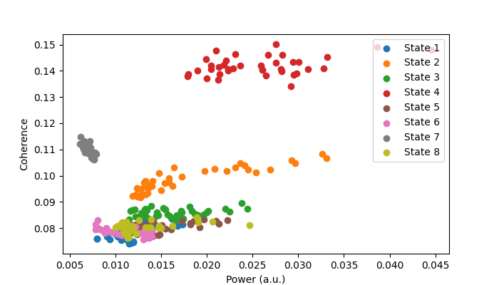
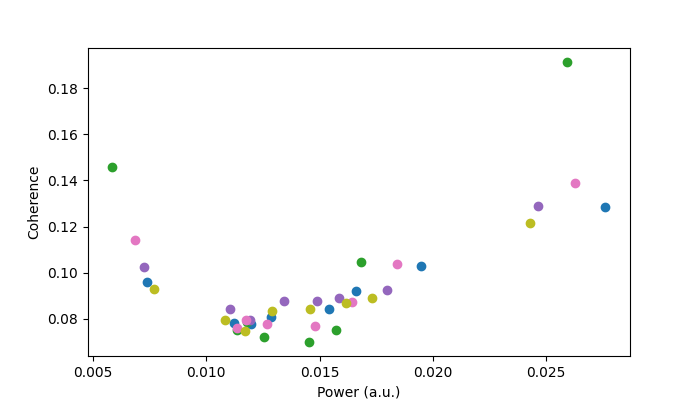
We can see the different states have different power/coherence properties. E.g. some states typically have more power/coherence at all parcels. If we average over subjects we get the following.

# Average power over parcels
mean_p = np.mean(p, axis=-1)
print(mean_p.shape)

# Average coherence over subjects
mean_c = np.mean(c, axis=(-2, -1))
print(mean_c.shape)

# Keep the first spectral component
mean_p = mean_p[:, 0]
mean_c = mean_c[:, 0]
print(mean_p.shape)
print(mean_c.shape)

# Plot
fig, ax = plotting.plot_scatter(
    mean_p,
    mean_c,
    x_label="Power (a.u.)",
    y_label="Coherence",
)

(5, 2, 8)
(5, 2, 8)
(5, 8)
(5, 8)

Each scatter point is a subject here. We also see different subjects have different power/coherence characteristics.

Total running time of the script: (2 minutes 24.134 seconds)

Gallery generated by Sphinx-Gallery