Static: Power Analysis

In this tutorial we will perform static power analysis on source space MEG data. This tutorial covers:

1. Getting the data

2. Calculating power from spectra

Getting the data

We will use resting-state MEG data that has already been source reconstructed. This dataset is:

• Parcellated to 38 regions of interest (ROI). The parcellation file used was atlas-Giles_nparc-38_space-MNI_res-8x8x8.nii.gz.

• Downsampled to 250 Hz.

• Bandpass filtered over the range 1-45 Hz.

Download the dataset

We will download example data hosted on OSF.

import os

def get_data(name, rename):
    os.system(f"osf -p by2tc fetch data/{name}.zip")
    os.makedirs(rename, exist_ok=True)
    os.system(f"unzip -o {name}.zip -d {rename}")
    os.remove(f"{name}.zip")
    return f"Data downloaded to: {rename}"

# Download the dataset (approximately 52 MB)
get_data("notts_meguk_giles_5_subjects", rename="source_data")

'Data downloaded to: source_data'

Load the data

We now load the data into osl-dynamics using the Data class. See the Loading Data tutorial for further details.

from osl_dynamics.data import Data

data = Data("source_data", n_jobs=4)
print(data)

QUEUEING TASKS | Loading files:   0%|          | 0/5 [00:00<?, ?it/s]
QUEUEING TASKS | Loading files: 100%|██████████| 5/5 [00:00<00:00, 5225.90it/s]

PROCESSING TASKS | Loading files:   0%|          | 0/5 [00:00<?, ?it/s]
PROCESSING TASKS | Loading files: 100%|██████████| 5/5 [00:00<00:00, 450.49it/s]

COLLECTING RESULTS | Loading files:   0%|          | 0/5 [00:00<?, ?it/s]
COLLECTING RESULTS | Loading files: 100%|██████████| 5/5 [00:00<00:00, 144631.17it/s]
Data
 id: 139852004548944
 n_sessions: 5
 n_samples: 371752
 n_channels: 38

For static analysis we just need the time series for the parcellated data. We can access this using the time_series method.

ts = data.time_series()

ts a list of numpy arrays. Each numpy array is a (n_samples, n_channels) time series for each subject.

Calculate spectra

First, we calculate the subject-specific power spectra. See the Static Power Spectra Analysis tutorial for more comprehensive description of power spectra analysis.

import numpy as np
from osl_dynamics.analysis import static

# Calculate power spectra
f, psd = static.welch_spectra(
    data=ts,
    sampling_frequency=250,
    window_length=500,
    standardize=True,
)

# Save
os.makedirs("spectra", exist_ok=True)
np.save("spectra/f.npy", f)
np.save("spectra/psd.npy", psd)

Calculating spectra:   0%|          | 0/5 [00:00<?, ?it/s]
Calculating spectra:  40%|████      | 2/5 [00:00<00:00, 12.56it/s]
Calculating spectra:  80%|████████  | 4/5 [00:00<00:00, 12.46it/s]
Calculating spectra: 100%|██████████| 5/5 [00:00<00:00, 12.45it/s]

Calculate power

Let’s first load the power spectra we previously calculated.

f = np.load("spectra/f.npy")
psd = np.load("spectra/psd.npy")

To understand these arrays it’s useful to print their shape:

print(f.shape)
print(psd.shape)

(251,)
(5, 38, 251)

We can see f is a 1D numpy array of length 256. This is the frequency axis of the power spectra. We can see psd is a subjects by channels (ROIs) by frequency array. E.g. psd[0] is a (38, 256) shaped array containing the power spectra for each of the 38 ROIs.

A useful property of a power spectrum is that the integral over a frequency range gives the power (or equivalently the variance of activity over the frequency range). osl-dynamics has a osl_dynamics.analysis.power module for performing power analyses.

Let’s say we are interested in alpha (10 Hz) power. We can calculate alpha power by integrating a power spectrum over a frequency range near 10 Hz. Typically, 7-13 Hz power is referred to as the ‘alpha band’. Other common frequency bands are:

• Delta: 1-4 Hz.

• Theta: 4-7 Hz.

• Beta: 13-30 Hz.

• Gamma: 30+ Hz.

osl-dynamics has a analysis.power.variance_from_spectra function to calculate power from a spectrum. Let’s use this function to calculate power for the alpha band.

from osl_dynamics.analysis import power

# Calculate power in the alpha band (8-12 Hz) from the spectra
p = power.variance_from_spectra(f, psd, frequency_range=[7, 13])

Note, if frequency_range is not passed, power.variance_from_spectra will integrate the power spectrum over all frequencies.

We can print the shape of the p array to help understand what is contained within it.

print(p.shape)

(5, 38)

From this, we can see it is a subjects by ROIs array. It has integrated the power spectrum for each ROI separately. If we wanted the alpha power at each ROI for the first subject, we would use p[0], which would be a (38,) shaped array.

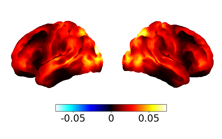
Plot power maps

We can use power.save to visualise the power maps. Let’s plot the group average.

group_p = np.mean(p, axis=0)

fig, ax = power.save(
    group_p,
    mask_file="MNI152_T1_8mm_brain.nii.gz",
    parcellation_file="atlas-Giles_nparc-38_space-MNI_res-8x8x8.nii.gz",
)

Saving images:   0%|          | 0/1 [00:00<?, ?it/s]
Saving images: 100%|██████████| 1/1 [00:00<00:00,  2.99it/s]
Saving images: 100%|██████████| 1/1 [00:00<00:00,  2.99it/s]

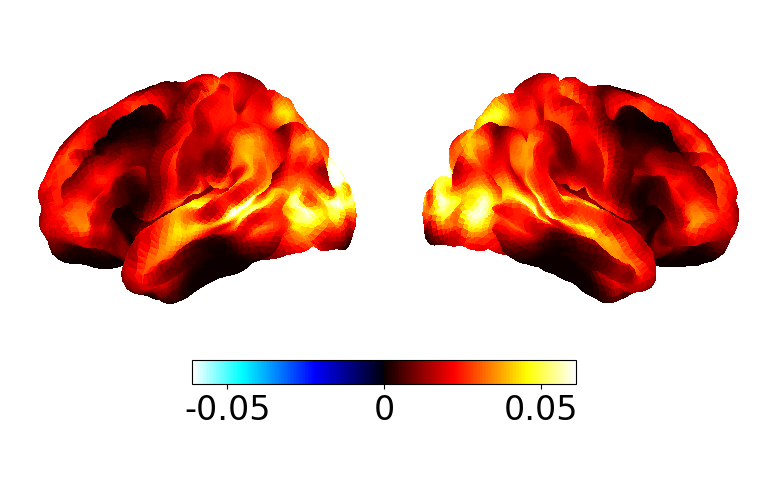
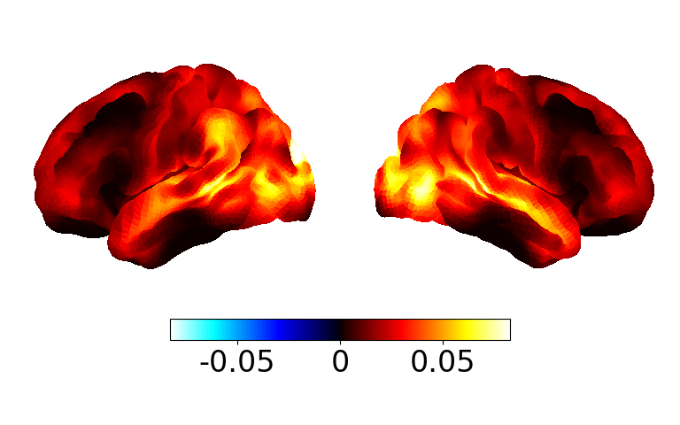
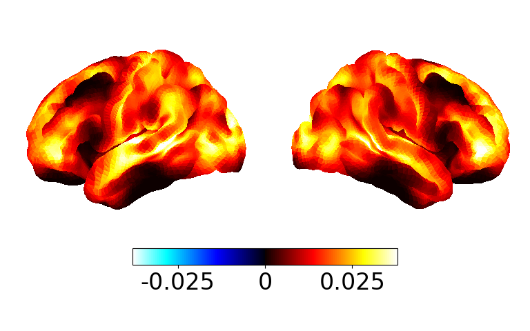
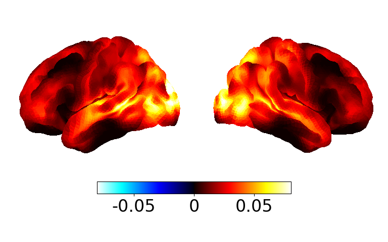
Or we can plot power maps for individual subjects, e.g.

fig, ax = power.save(
    p[:4],  # first four
    mask_file="MNI152_T1_8mm_brain.nii.gz",
    parcellation_file="atlas-Giles_nparc-38_space-MNI_res-8x8x8.nii.gz",
)

• 
• 
• 
• 

Saving images:   0%|          | 0/4 [00:00<?, ?it/s]
Saving images:  25%|██▌       | 1/4 [00:00<00:01,  2.85it/s]
Saving images:  50%|█████     | 2/4 [00:00<00:00,  2.80it/s]
Saving images:  75%|███████▌  | 3/4 [00:01<00:00,  2.76it/s]
Saving images: 100%|██████████| 4/4 [00:01<00:00,  2.70it/s]
Saving images: 100%|██████████| 4/4 [00:01<00:00,  2.73it/s]