Static: Spectral Analysis

MEG data is useful because it has a high temporal resolution. We can take advantage of this by examining the spectral (i.e. frequency) content of the data. In this tutorial we will perform static spectral analysis on source space MEG data. This tutorial covers:

1. Getting the data

2. Calculating spectra for each subject

Getting the data

We will use resting-state MEG data that has already been source reconstructed. This dataset is:

• Parcellated to 38 regions of interest (ROI). The parcellation file used was atlas-Giles_nparc-38_space-MNI_res-8x8x8.nii.gz.

• Downsampled to 250 Hz.

• Bandpass filtered over the range 1-45 Hz.

Download the dataset

We will download example data hosted on OSF.

import os

def get_data(name, rename):
    os.system(f"osf -p by2tc fetch data/{name}.zip")
    os.makedirs(rename, exist_ok=True)
    os.system(f"unzip -o {name}.zip -d {rename}")
    os.remove(f"{name}.zip")
    return f"Data downloaded to: {rename}"

# Download the dataset (approximately 52 MB)
get_data("notts_meguk_giles_5_subjects", rename="source_data")

'Data downloaded to: source_data'

Load the data

We now load the data into osl-dynamics using the Data class. See the Loading Data tutorial for further details.

from osl_dynamics.data import Data

data = Data("source_data", n_jobs=4)
print(data)

QUEUEING TASKS | Loading files:   0%|          | 0/5 [00:00<?, ?it/s]
QUEUEING TASKS | Loading files: 100%|██████████| 5/5 [00:00<00:00, 1083.63it/s]

PROCESSING TASKS | Loading files:   0%|          | 0/5 [00:00<?, ?it/s]
PROCESSING TASKS | Loading files: 100%|██████████| 5/5 [00:00<00:00, 344.46it/s]

COLLECTING RESULTS | Loading files:   0%|          | 0/5 [00:00<?, ?it/s]
COLLECTING RESULTS | Loading files: 100%|██████████| 5/5 [00:00<00:00, 124830.48it/s]
Data
 id: 139852003221072
 n_sessions: 5
 n_samples: 371752
 n_channels: 38

For static analysis we just need the time series for the parcellated data. We can access this using the time_series method.

ts = data.time_series()

ts a list of numpy arrays. Each numpy array is a (n_samples, n_channels) time series for each subject.

Subject-Level Analysis

In this section, we will ignore the fact this data was collected in a task paradigm and will just aim to study the power spectrum of each subject.

Calculate power spectra

Using the data we just loaded, we want to calculate the power spectra for each channel (ROI) for each subject. We will use the osl_dynamics.analysis.static.welch_spectra() function to do this. This function implements Welch’s methods for calculating power spectra.

To use this function we need to specify at least two arguments:

• sampling_frequency. This is to ensure we get the correct frequency axis for the power spectra.

• window_length. This is the number of samples in the sliding window. The longer the window the smaller the frequency resolution of the power spectrum. Twice the sampling frequency is generally a good choice for this, which gives a frequency resolution of 0.5 Hz.

We can also specify an optional argument:

• standardize. This will z-score the data (for each subejct separately) before calculate the power spectra. This can be helpful if you want to examine power the fraction of power in a frequency band relative to the total power (across all frequencies) of the subject.

from osl_dynamics.analysis import static

f, psd = static.welch_spectra(
    data=ts,
    sampling_frequency=250,
    window_length=500,
    standardize=True,
)

Calculating spectra:   0%|          | 0/5 [00:00<?, ?it/s]
Calculating spectra:  40%|████      | 2/5 [00:00<00:00, 12.42it/s]
Calculating spectra:  80%|████████  | 4/5 [00:00<00:00, 12.37it/s]
Calculating spectra: 100%|██████████| 5/5 [00:00<00:00, 12.38it/s]

We have two numpy arrays: f, which is the frequency axis of the power spectra in Hz, and p, which contains the power spectra.

Calculating power spectra can be time consuming. We will want to use the power spectra many times to make different plots. We don’t want to have to calculate them repeatedly, so often it is convenient to save the f and p numpy arrays so we can load them later (instead of calculating them again). Let’s save the spectra.

import numpy as np

os.makedirs("spectra", exist_ok=True)
np.save("spectra/f.npy", f)
np.save("spectra/psd.npy", psd)

Plot the power spectra

Let’s first load the power spectra we previously calculated.

f = np.load("spectra/f.npy")
psd = np.load("spectra/psd.npy")

To understand these arrays it’s useful to print their shape:

print(f.shape)
print(psd.shape)

(251,)
(5, 38, 251)

We can see f is a 1D numpy array of length 256. This is the frequency axis of the power spectra. We can see psd is a subjects by channels (ROIs) by frequency array. E.g. psd[0] is a (38, 256) shaped array containing the power spectra for each of the 38 ROIs.

Let’s plot the power spectrum for each ROI for the first subject. We will use the osl_dynamics.utils.plotting module to do the basic plotting. See the Plotting tutorial for further info.

from osl_dynamics.utils import plotting

fig, ax = plotting.plot_line(
    [f] * psd.shape[1],
    psd[0],
    x_label="Frequency (Hz)",
    y_label="PSD (a.u.)",
)

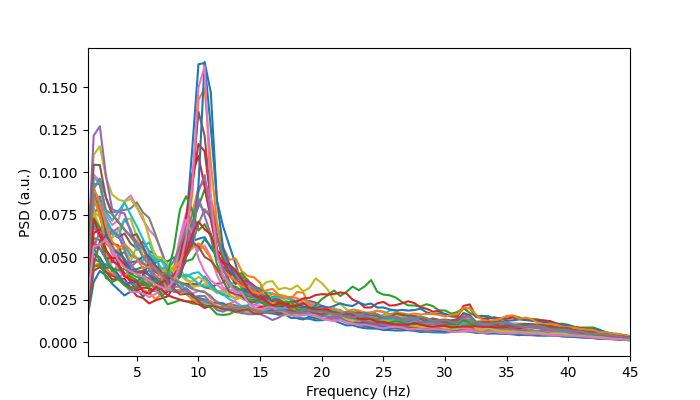
Each line in this plot is a ROI. We can see there’s a lot of activity in the 1-20 Hz range. Let’s zoom into the 1-45 Hz range.

fig, ax = plotting.plot_line(
    [f] * psd.shape[1],
    psd[0],
    x_label="Frequency (Hz)",
    y_label="PSD (a.u.)",
    x_range=[1, 45],
)

Note, if you wanted to save this as an image you could pass a filename=”<filename>.png” argument to this function. All functions in osl_dynamics.utils.plotting have this argument.

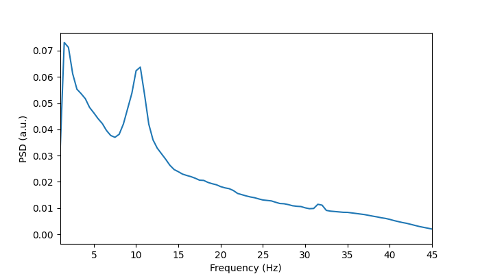
Rather than plotting the power spectrum for each ROI, let’s average over channels to give a single line for each subject.

# Average over channels
psd_mean = np.mean(psd, axis=1)

# Plot the mean power spectrum for the first subject
fig, ax = plotting.plot_line(
    [f],
    [psd_mean[0]],
    x_label="Frequency (Hz)",
    y_label="PSD (a.u.)",
    x_range=[1, 45],
)

We can add a shaded area around the solid line to give an idea of the variability around the mean.

# Standard deviation around the mean
psd_std = np.std(psd, axis=1)

# Plot with one sigma shaded
fig, ax = plotting.plot_line(
    [f],
    [psd_mean[0]],
    errors=[[psd_mean[0] - psd_std[0]], [psd_mean[0] + psd_std[0]]],
    x_label="Frequency (Hz)",
    y_label="PSD (a.u.)",
    x_range=[1, 45],
)

Finally, let’s plot the average power spectrum for each subject in the same figure.

fig, ax = plotting.plot_line(
    [f] * psd.shape[0],
    psd_mean,
    x_label="Frequency (Hz)",
    y_label="PSD (a.u.)",
    x_range=[1, 45],
)

We can see there’s quite a bit of variation in the static power spectrum for each subject. Some subjects have a pronounced alpha (around 10 Hz) peak. Some subjects have high beta (around 20 Hz) activity, others don’t.