
Note
Go to the end to download the full example code.
Time-Delay Embedding#
In this tutorial we will explore the impact of different settings for time-delay embedding (n_embeddings) and the number of principal component analysis (PCA) components (n_pca_components).
Time-delay embedding (TDE) is a process of augmenting a time series with extra channels. These extra channels are time-lagged versions of the original channels. We do this to add extra entries to the covariance matrix of the data which are sensitive to the frequency of oscillations in the data. To understand this better, let’s simulate some sinusoidal data.
import numpy as np
import matplotlib.pyplot as plt

# Simulate data:
# - Channel 1: 10 Hz sine wave
# - Channel 2: 20 Hz sine wave
# - Channel 3: 20 Hz sine wave synchronised with channel 2 but with different amplitude
n = 10000
t = np.arange(n) / 200  # we're using a sampling frequency of 200 Hz
p = np.random.uniform(0, 2 * np.pi, size=(2,))  # random phases
x = np.array([
    1.0 * np.sin(2 * np.pi * 10 * t + p[0]),
    1.5 * np.sin(2 * np.pi * 20 * t + p[1]),
    0.6 * np.sin(2 * np.pi * 20 * t + p[1]),  # same phase as channel 2
])

# Add some noise
x += np.random.normal(0, 0.1, size=x.shape)

# Plot first 0.2 s
fig, ax = plt.subplots(nrows=3, ncols=1)
ax[0].plot(t[:40], x[0,:40], label="Channel 1")
ax[1].plot(t[:40], x[1,:40], label="Channel 2")
ax[2].plot(t[:40], x[2,:40], label="Channel 3")
ax[0].set_ylabel("Channel 1")
ax[1].set_ylabel("Channel 2")
ax[2].set_ylabel("Channel 3")
ax[2].set_xlabel("Time (s)")
plt.tight_layout()

Let’s plot the covariance of this data.
cov = np.cov(x)

plt.matshow(cov)
plt.colorbar()

<matplotlib.colorbar.Colorbar object at 0x716ecf149460>
The covariance here is a 3x3 matrix because we have 3 channels. The diagonal of this matrix is the variance and reflects the amplitude of each sine wave. The off-diagonal elements reflect the covariance between channels. In this example the covariance between the channels 1 and 2 is close to zero, however there is some covariance between channels 2 and 3 due to the phase synchronisation. Let’s see what happens to the covariance matrix when we TDE the data.
from osl_dynamics.data import Data

# First load the data into osl-dynamics
data = Data(x, time_axis_first=False)
print(data)

# Perform time-delay embedding
data.tde(n_embeddings=5)
Loading files:   0%|          | 0/1 [00:00<?, ?it/s]
Loading files: 100%|██████████| 1/1 [00:00<00:00, 18558.87it/s]
Data
 id: 124720711796880
 n_sessions: 1
 n_samples: 10000
 n_channels: 3

TDE:   0%|          | 0/1 [00:00<?, ?it/s]
TDE: 100%|██████████| 1/1 [00:00<00:00, 2568.47it/s]

<osl_dynamics.data.base.Data object at 0x716ecdb90890>
See the Data loading tutorial for further details regarding how to load data using the osl_dynamics.data.base.Data class. In the above code we chose n_embeddings=5. This means for every original channel, we add n_embeddings - 1 = 4 extra channels. In our three channel example, the operation we do is:
\(\begin{pmatrix} x(t) \\ y(t) \\ z(t) \end{pmatrix} \rightarrow \begin{pmatrix} x(t-2) \\ x(t-1) \\ x(t) \\ x(t+1) \\ x(t+2) \\ y(t-2) \\ y(t-1) \\ y(t) \\ y(t+1) \\ y(t+2) \\ z(t-2) \\ z(t-1) \\ z(t) \\ z(t+1) \\ z(t+2) \end{pmatrix}\)
We should expect a total of n_embeddings * 3 channels, in our example this is 5 * 3 = 15. We can verify this by printing the Data object.
print(data)
Data
 id: 124720711796880
 n_sessions: 1
 n_samples: 9996
 n_channels: 15
We can see we have 15 channels as expected. Note, we have also lost n_embeddings - 1 = 4 time points (we have 9996 samples when originally we simulated 10000). This is because we don’t have the full window to TDE the time points at the start and end of the time series.
Let’s look at the covariance of the TDE data.
cov_tde = np.cov(data.time_series(), rowvar=False)

plt.matshow(cov_tde)
plt.colorbar()

<matplotlib.colorbar.Colorbar object at 0x716ecd86c140>
This covariance matrix is 15x15 because we have 15 channels. The blocks on the diagonal of the above matrix represents the covariance of a channel with a time-lagged version of itself - this quantity is known as the auto-correlation function. Blocks on the off-diagonal represent the covariance of a channel with a time-lagged version of another channel - this quantity is known as the cross-correlation function.
We can extract an estimate of the auto/cross-correlation function (A/CCF) by taking values from this covariance matrix. osl-dynamics has a function we can use for this: osl_dynamics.analysis.post_hoc.autocorr_from_tde_cov(). This function will extract both ACFs and CCFs from a TDE covariance matrix.
from osl_dynamics.analysis import post_hoc, spectral

# Extract A/CCFs from the covariance
tau, acf = post_hoc.autocorr_from_tde_cov(cov_tde, n_embeddings=5)
print(acf.shape)  # channels x channels x time lags

# Plot ACFs
plt.plot(tau, acf[0,0], label="Channel 1")
plt.plot(tau, acf[1,1], label="Channel 2")
plt.plot(tau, acf[2,2], label="Channel 3")
plt.xlabel("Time Lag (Samples)")
plt.ylabel("ACF (a.u)")
plt.legend()
plt.tight_layout()

(3, 3, 9)
The diagonal of acf represents the ACF, e.g. acf[0,0] is the ACF for for channel 1 (indexed by 0). The off-diagonal of acf represent the CCF, e.g. acf[0,1] is the CCF for channel 1 and 2.
The ACF and power spectral density (PSD) form a Fourier pair. This means we can calculate an estimate of the PSD of each channel by Fourier transforming the ACF. Let’s do this using the osl_dynamics.analysis.spectral.autocorr_to_spectra() function in osl-dynamics. Note, this function will also calculate cross PSD using the CCFs.
# Calculate PSD by Fourier transforming the ACF
f, psd, _ = spectral.autocorr_to_spectra(acf, sampling_frequency=200)
print(psd.shape)  # channels x channels x frequency

# Plot
plt.plot(f, psd[0,0], label="Channel 1")
plt.plot(f, psd[1,1], label="Channel 2")
plt.plot(f, psd[2,2], label="Channel 3")
plt.xlabel("Frequency (Hz)")
plt.ylabel("PSD (a.u)")
plt.legend()

(3, 3, 33)

<matplotlib.legend.Legend object at 0x716ecd964770>
We can see the 20 Hz peak in the channel 2, which corresponds well to what we simulated. We also see a smaller 20 Hz peak for channel 3. However, we aren’t able to resolve the 10 Hz peak we simulated for channel 1. This was because we didn’t use enough lags to resolve the 10 Hz peak.
Note, we can see some ringing, this is due to padding the ACF with zeros (to obtain an integer multiple of 2) before calculating the Fourier transform, we can change the padding via the nfft argument to osl_dynamics.analysis.spectral.autocorr_to_spectra().
Let’s try again with more lags - this will mean we evaluate the ACF for a greater window of time lags, this will result in a higher resolution PSD.
# Redo the TDE on the original data
data.tde(n_embeddings=11, use_raw=True)
print(data)

# Calculate TDE covariance, ACF and PSD
cov_tde = np.cov(data.time_series(), rowvar=False)
tau, acf = post_hoc.autocorr_from_tde_cov(cov_tde, n_embeddings=11)
f, psd, _ = spectral.autocorr_to_spectra(acf, sampling_frequency=200)

# Plot
fig, ax = plt.subplots(nrows=1, ncols=3, figsize=(10, 3))
ax[0].matshow(cov_tde)

ax[1].plot(tau, acf[0,0])
ax[1].plot(tau, acf[1,1])
ax[1].plot(tau, acf[2,2])
ax[1].set_xlabel("Time Lag (Samples)")
ax[1].set_ylabel("ACF (a.u.)")

ax[2].plot(f, psd[0,0], label="Channel 1")
ax[2].plot(f, psd[1,1], label="Channel 2")
ax[2].plot(f, psd[2,2], label="Channel 2")
ax[2].set_xlabel("Frequency (Hz)")
ax[2].set_ylabel("PSD (a.u.)")
ax[2].legend()
plt.tight_layout()

TDE:   0%|          | 0/1 [00:00<?, ?it/s]
TDE: 100%|██████████| 1/1 [00:00<00:00, 2020.38it/s]
Data
 id: 124720711796880
 n_sessions: 1
 n_samples: 9990
 n_channels: 33
We can see the ACF extends over a wider range and we’re now able to better model the 10 Hz sine wave in channel 1. We can also see what happens if we change the frequency of the sine wave for channel 1. Let’s simulate a 30 Hz sine wave for channel 1.
# Simulate new data
x = np.array([
    1.0 * np.sin(2 * np.pi * 30 * t + p[0]),  # 30 Hz
    1.5 * np.sin(2 * np.pi * 20 * t + p[1]),
    0.6 * np.sin(2 * np.pi * 20 * t + p[1]),  # same phase as channel 2
])
x += np.random.normal(0, 0.15, size=x.shape)
data = Data(x, time_axis_first=False)

# TDE
data.tde(n_embeddings=11)

# Calculate TDE covariance, ACF and PSD
cov_tde = np.cov(data.time_series(), rowvar=False)
tau, acf = post_hoc.autocorr_from_tde_cov(cov_tde, n_embeddings=11)
f, psd, _ = spectral.autocorr_to_spectra(acf, sampling_frequency=200)

# Plot
fig, ax = plt.subplots(nrows=1, ncols=3, figsize=(10, 3))
ax[0].matshow(cov_tde)

ax[1].plot(tau, acf[0,0])
ax[1].plot(tau, acf[1,1])
ax[1].plot(tau, acf[2,2])
ax[1].set_xlabel("Time Lag (Samples)")
ax[1].set_ylabel("ACF (a.u.)")

ax[2].plot(f, psd[0,0], label="Channel 1")
ax[2].plot(f, psd[1,1], label="Channel 2")
ax[2].plot(f, psd[2,2], label="Channel 2")
ax[2].set_xlabel("Frequency (Hz)")
ax[2].set_ylabel("PSD (a.u.)")
ax[2].legend()
plt.tight_layout()

Loading files:   0%|          | 0/1 [00:00<?, ?it/s]
Loading files: 100%|██████████| 1/1 [00:00<00:00, 18808.54it/s]

TDE:   0%|          | 0/1 [00:00<?, ?it/s]
TDE: 100%|██████████| 1/1 [00:00<00:00, 2081.54it/s]
We can see the covariance of the TDE data, as well as the ACF/PSD has, changed to reflect the frequency of data. The above example shows how TDE leads to covariance matrices that are sensitive to oscillatory frequencies in the original data and how the number of embeddings relates to the frequency resolution that can be modelled.
In addition to modelling the frequency of oscillations in an individual channel, we can also model phase synchronisation across channels using TDE data. We can see from the above TDE covariance matrix the off-diagonal block for channels 2 and 3 (row 10-20, column 20-30) shows some structure. Let’s plot the CCF for each pair of channels.
plt.plot(tau, acf[0,1], label="Channel 1+2")
plt.plot(tau, acf[1,2], label="Channel 2+3")
plt.xlabel("Time Lag (Samples)")
plt.ylabel("CCF (a.u.)")
plt.legend()

<matplotlib.legend.Legend object at 0x716ecaf64770>
The structure in the CCF for channels 2 and 3 shows the time-lagged versions of these channels are correlated. Such structure arises from phase synchronisation. In contrast, we don’t see any structure for the CCF between channels 1 and 2. This is because we simulated random phases for these channels.
Let’s plot the cross PSD for these channels.
plt.plot(f, psd[0,1], label="Channel 1+2")
plt.plot(f, psd[1,2], label="Channel 2+3")
plt.xlabel("Frequency (Hz)")
plt.ylabel("Cross PSD (a.u)")
plt.legend()

<matplotlib.legend.Legend object at 0x716ec823e360>
We can see the cross PSD indicates the frequencies which show phase synchronisation.
In the above examples we have shown how the covariance of TDE data can capture the oscillatory properties (power spectra and frequency-specific coupling) of a time series.
Impact of different parameters#
When we apply TDE-PCA, we need to specify the number of embeddings and PCA components. The number of embeddings affects the frequencies we are able to distinguish in the data. To demonstrate we can simulate sinusoidal data and apply TDE.
from osl_dynamics.analysis import spectral

def calc_covs_psds(frequencies, n_embeddings, fs):
    covs = []
    psds = []
    t = np.arange(1000) / fs
    for F in frequencies:
        x = np.sin(2 * np.pi * F * t)[:, np.newaxis]
        data = Data(x)
        data.prepare({
            "tde": {"n_embeddings": n_embeddings},
            "standardize": {},
        })
        cov = np.cov(data.time_series(), rowvar=False)
        tau, acf = post_hoc.autocorr_from_tde_cov(cov, n_embeddings=n_embeddings)
        f, p, _ = spectral.autocorr_to_spectra(
            acf[np.newaxis, np.newaxis, :],
            sampling_frequency=fs,
        )
        covs.append(cov)
        psds.append(p)
    return covs, psds

frequencies = [1, 4, 8, 13, 20, 30, 40]
n_embeddings = 5
fs = 250

covs, psds = calc_covs_psds(frequencies, n_embeddings, fs)
Loading files:   0%|          | 0/1 [00:00<?, ?it/s]
Loading files: 100%|██████████| 1/1 [00:00<00:00, 26886.56it/s]

TDE:   0%|          | 0/1 [00:00<?, ?it/s]
TDE: 100%|██████████| 1/1 [00:00<00:00, 6482.70it/s]

Standardize:   0%|          | 0/1 [00:00<?, ?it/s]
Standardize: 100%|██████████| 1/1 [00:00<00:00, 4006.02it/s]

Loading files:   0%|          | 0/1 [00:00<?, ?it/s]
Loading files: 100%|██████████| 1/1 [00:00<00:00, 33554.43it/s]

TDE:   0%|          | 0/1 [00:00<?, ?it/s]
TDE: 100%|██████████| 1/1 [00:00<00:00, 7256.58it/s]

Standardize:   0%|          | 0/1 [00:00<?, ?it/s]
Standardize: 100%|██████████| 1/1 [00:00<00:00, 5377.31it/s]

Loading files:   0%|          | 0/1 [00:00<?, ?it/s]
Loading files: 100%|██████████| 1/1 [00:00<00:00, 34379.54it/s]

TDE:   0%|          | 0/1 [00:00<?, ?it/s]
TDE: 100%|██████████| 1/1 [00:00<00:00, 7710.12it/s]

Standardize:   0%|          | 0/1 [00:00<?, ?it/s]
Standardize: 100%|██████████| 1/1 [00:00<00:00, 5440.08it/s]

Loading files:   0%|          | 0/1 [00:00<?, ?it/s]
Loading files: 100%|██████████| 1/1 [00:00<00:00, 36157.79it/s]

TDE:   0%|          | 0/1 [00:00<?, ?it/s]
TDE: 100%|██████████| 1/1 [00:00<00:00, 7898.88it/s]

Standardize:   0%|          | 0/1 [00:00<?, ?it/s]
Standardize: 100%|██████████| 1/1 [00:00<00:00, 5540.69it/s]

Loading files:   0%|          | 0/1 [00:00<?, ?it/s]
Loading files: 100%|██████████| 1/1 [00:00<00:00, 35246.25it/s]

TDE:   0%|          | 0/1 [00:00<?, ?it/s]
TDE: 100%|██████████| 1/1 [00:00<00:00, 7913.78it/s]

Standardize:   0%|          | 0/1 [00:00<?, ?it/s]
Standardize: 100%|██████████| 1/1 [00:00<00:00, 3160.74it/s]

Loading files:   0%|          | 0/1 [00:00<?, ?it/s]
Loading files: 100%|██████████| 1/1 [00:00<00:00, 35246.25it/s]

TDE:   0%|          | 0/1 [00:00<?, ?it/s]
TDE: 100%|██████████| 1/1 [00:00<00:00, 8019.70it/s]

Standardize:   0%|          | 0/1 [00:00<?, ?it/s]
Standardize: 100%|██████████| 1/1 [00:00<00:00, 4588.95it/s]

Loading files:   0%|          | 0/1 [00:00<?, ?it/s]
Loading files: 100%|██████████| 1/1 [00:00<00:00, 35848.75it/s]

TDE:   0%|          | 0/1 [00:00<?, ?it/s]
TDE: 100%|██████████| 1/1 [00:00<00:00, 7943.76it/s]

Standardize:   0%|          | 0/1 [00:00<?, ?it/s]
Standardize: 100%|██████████| 1/1 [00:00<00:00, 4629.47it/s]
Let’s plot the covariance of the TDE data and corresponding PSD for these different sine waves.
def plot_covs_psds(covs, psds):
    fig, ax = plt.subplots(nrows=2, ncols=len(psds), figsize=(12,3))
    for i in range(len(psds)):
        ax[0, i].set_title(f"f={frequencies[i]} Hz")
        ax[0, i].imshow(covs[i])
        ax[0, i].axis("off")
        ax[1, i].plot(f, psds[i])
        ax[1, i].set_xlim(1, 45)
        ax[1, i].set_ylim(0, np.max(psds))
        ax[1, i].set_xlabel("Frequency (Hz)")
    ax[1, 0].set_ylabel("PSD (a.u.)")
    plt.tight_layout()

plot_covs_psds(covs, psds)
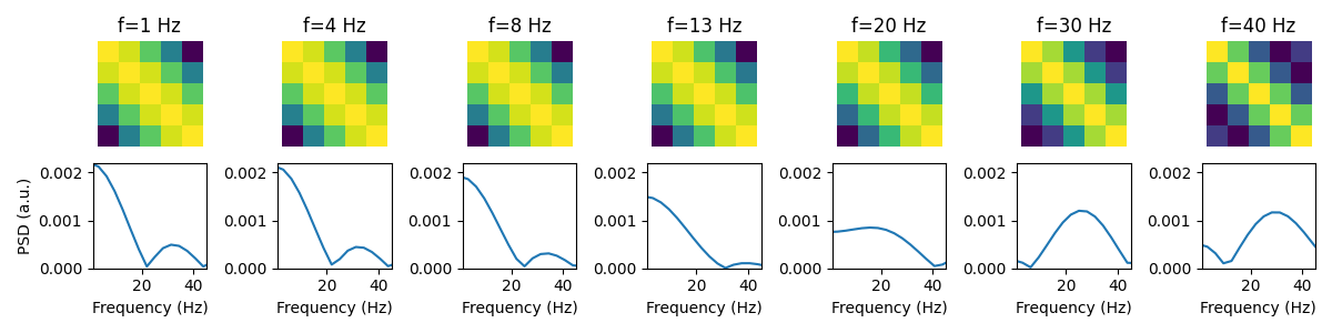
We can see despite using a small number of embeddings we are sensitive to a changes in a wide range of frequencies. However, we see we strugle to distinguish between low frequencies. We can improve the frequency resolution by increasing the number of embeddings. Let’s do
frequencies = [1, 4, 8, 13, 20, 30, 40]
n_embeddings = 11
fs = 250

covs, psds = calc_covs_psds(frequencies, n_embeddings, fs)
plot_covs_psds(covs, psds)

Loading files:   0%|          | 0/1 [00:00<?, ?it/s]
Loading files: 100%|██████████| 1/1 [00:00<00:00, 25731.93it/s]

TDE:   0%|          | 0/1 [00:00<?, ?it/s]
TDE: 100%|██████████| 1/1 [00:00<00:00, 6355.01it/s]

Standardize:   0%|          | 0/1 [00:00<?, ?it/s]
Standardize: 100%|██████████| 1/1 [00:00<00:00, 4534.38it/s]

Loading files:   0%|          | 0/1 [00:00<?, ?it/s]
Loading files: 100%|██████████| 1/1 [00:00<00:00, 33026.02it/s]

TDE:   0%|          | 0/1 [00:00<?, ?it/s]
TDE: 100%|██████████| 1/1 [00:00<00:00, 7516.67it/s]

Standardize:   0%|          | 0/1 [00:00<?, ?it/s]
Standardize: 100%|██████████| 1/1 [00:00<00:00, 4888.47it/s]

Loading files:   0%|          | 0/1 [00:00<?, ?it/s]
Loading files: 100%|██████████| 1/1 [00:00<00:00, 20460.02it/s]

TDE:   0%|          | 0/1 [00:00<?, ?it/s]
TDE: 100%|██████████| 1/1 [00:00<00:00, 6186.29it/s]

Standardize:   0%|          | 0/1 [00:00<?, ?it/s]
Standardize: 100%|██████████| 1/1 [00:00<00:00, 4969.55it/s]

Loading files:   0%|          | 0/1 [00:00<?, ?it/s]
Loading files: 100%|██████████| 1/1 [00:00<00:00, 33825.03it/s]

TDE:   0%|          | 0/1 [00:00<?, ?it/s]
TDE: 100%|██████████| 1/1 [00:00<00:00, 7839.82it/s]

Standardize:   0%|          | 0/1 [00:00<?, ?it/s]
Standardize: 100%|██████████| 1/1 [00:00<00:00, 5023.12it/s]

Loading files:   0%|          | 0/1 [00:00<?, ?it/s]
Loading files: 100%|██████████| 1/1 [00:00<00:00, 20164.92it/s]

TDE:   0%|          | 0/1 [00:00<?, ?it/s]
TDE: 100%|██████████| 1/1 [00:00<00:00, 7958.83it/s]

Standardize:   0%|          | 0/1 [00:00<?, ?it/s]
Standardize: 100%|██████████| 1/1 [00:00<00:00, 4346.43it/s]

Loading files:   0%|          | 0/1 [00:00<?, ?it/s]
Loading files: 100%|██████████| 1/1 [00:00<00:00, 33825.03it/s]

TDE:   0%|          | 0/1 [00:00<?, ?it/s]
TDE: 100%|██████████| 1/1 [00:00<00:00, 8128.50it/s]

Standardize:   0%|          | 0/1 [00:00<?, ?it/s]
Standardize: 100%|██████████| 1/1 [00:00<00:00, 4315.13it/s]

Loading files:   0%|          | 0/1 [00:00<?, ?it/s]
Loading files: 100%|██████████| 1/1 [00:00<00:00, 34663.67it/s]

TDE:   0%|          | 0/1 [00:00<?, ?it/s]
TDE: 100%|██████████| 1/1 [00:00<00:00, 7796.10it/s]

Standardize:   0%|          | 0/1 [00:00<?, ?it/s]
Standardize: 100%|██████████| 1/1 [00:00<00:00, 4917.12it/s]
We can see with 11 embeddings, we can get much sharper peaks in the PSD. Note, the sensitivity to different frequencies also depends on the sampling frequency. We advise making the above plots for the sampling frequency you have and ensure you have a high enough number of emebdding to give sufficient frequency resolution.
The number of embeddings will also depend on the PCA step that’s normally performed after TDE. The higher the number of embeddings the more PCA components you will need to retain high frequency oscillations. Let’s explore this further using real data.
Download the dataset#
We will download example data hosted on OSF.
import os

def get_data(name):
    os.system(f"osf -p by2tc fetch data/{name}.zip")
    os.system(f"unzip -o {name}.zip -d {name}")
    os.remove(f"{name}.zip")
    return f"Data downloaded to: {name}"

# Download the dataset (approximately 6 MB)
get_data("example_loading_data")

# List the contents of the downloaded directory containing the dataset
print("Contents of example_loading_data:")
os.listdir("example_loading_data")
Contents of example_loading_data:

['txt_format', 'matlab_format', 'fif_format', 'numpy_format']
Let’s load the data in numpy format. See the Loading Data tutorial for further details.
from osl_dynamics.data import Data

data = Data("example_loading_data/numpy_format", sampling_frequency=250)
print(data)
Loading files:   0%|          | 0/2 [00:00<?, ?it/s]
Loading files: 100%|██████████| 2/2 [00:00<00:00, 2829.21it/s]
Data
 id: 124720665688880
 n_sessions: 2
 n_samples: 12000
 n_channels: 42
We can see we have data for two subjects.
Apply TDE and PCA#
Both TDE and PCA can be done in one step using the tde_pca method. We often also want to standardize (z-score) the data before training a model. Both of these steps can be done with the prepare method.
methods = {
    "tde_pca": {"n_embeddings": 15, "n_pca_components": 80},
    "standardize": {},
}
data.prepare(methods)
print(data)
Calculating PCA components:   0%|          | 0/2 [00:00<?, ?it/s]
Calculating PCA components: 100%|██████████| 2/2 [00:00<00:00, 29.61it/s]

TDE-PCA:   0%|          | 0/2 [00:00<?, ?it/s]
TDE-PCA: 100%|██████████| 2/2 [00:00<00:00, 50.43it/s]

Standardize:   0%|          | 0/2 [00:00<?, ?it/s]
Standardize: 100%|██████████| 2/2 [00:00<00:00, 732.50it/s]
Data
 id: 124720665688880
 n_sessions: 2
 n_samples: 11972
 n_channels: 80
We can see the n_samples attribute of our Data object has changed from 147500 to 147472. We have lost 28 samples. This is due to the TDE. We lose n_embeddings // 2 data points from each end of the time series for each subject. In other words, with n_embeddings=15, we lose the first 7 and last 7 data points from each subject. We lose a total of 28 data points because we have 2 subjects.
Scan different parameters#
Let calculate the PSD of prepared data using different parameters for TDE-PCA.
def calc_psds(n_time_embeddings, n_pca_components, fs):
    psds = []
    for i, n_tde in enumerate(n_time_embeddings):
        psds.append([])
        for n_pca in n_pca_components:
            methods = {
                "tde_pca": {"n_embeddings": n_tde, "n_pca_components": n_pca, "use_raw": True},
                "standardize": {},
            }
            data.prepare(methods)
            f, psd = spectral.welch_spectra(
                data.time_series(concatenate=True),
                sampling_frequency=fs,
                frequency_range=[1, 45],
                calc_coh=False,
            )
            p = np.mean(psd, axis=0)  # average over channels
            psds[-1].append(p)
    return f, psds

n_time_embeddings = [7, 11, 15, 19]
n_pca_components = [40, 60, 80, 100, 120, 140]
fs = 250

f, psds = calc_psds(n_time_embeddings, n_pca_components, fs)
Calculating PCA components:   0%|          | 0/2 [00:00<?, ?it/s]
Calculating PCA components: 100%|██████████| 2/2 [00:00<00:00, 51.06it/s]

TDE-PCA:   0%|          | 0/2 [00:00<?, ?it/s]
TDE-PCA: 100%|██████████| 2/2 [00:00<00:00, 154.82it/s]

Standardize:   0%|          | 0/2 [00:00<?, ?it/s]
Standardize: 100%|██████████| 2/2 [00:00<00:00, 951.95it/s]

Calculating PCA components:   0%|          | 0/2 [00:00<?, ?it/s]
Calculating PCA components: 100%|██████████| 2/2 [00:00<00:00, 85.32it/s]

TDE-PCA:   0%|          | 0/2 [00:00<?, ?it/s]
TDE-PCA: 100%|██████████| 2/2 [00:00<00:00, 136.80it/s]

Standardize:   0%|          | 0/2 [00:00<?, ?it/s]
Standardize: 100%|██████████| 2/2 [00:00<00:00, 760.46it/s]

Calculating PCA components:   0%|          | 0/2 [00:00<?, ?it/s]
Calculating PCA components: 100%|██████████| 2/2 [00:00<00:00, 85.30it/s]

TDE-PCA:   0%|          | 0/2 [00:00<?, ?it/s]
TDE-PCA: 100%|██████████| 2/2 [00:00<00:00, 133.12it/s]

Standardize:   0%|          | 0/2 [00:00<?, ?it/s]
Standardize: 100%|██████████| 2/2 [00:00<00:00, 752.07it/s]

Calculating PCA components:   0%|          | 0/2 [00:00<?, ?it/s]
Calculating PCA components: 100%|██████████| 2/2 [00:00<00:00, 85.04it/s]

TDE-PCA:   0%|          | 0/2 [00:00<?, ?it/s]
TDE-PCA: 100%|██████████| 2/2 [00:00<00:00, 120.51it/s]

Standardize:   0%|          | 0/2 [00:00<?, ?it/s]
Standardize: 100%|██████████| 2/2 [00:00<00:00, 632.91it/s]

Calculating PCA components:   0%|          | 0/2 [00:00<?, ?it/s]
Calculating PCA components: 100%|██████████| 2/2 [00:00<00:00, 85.49it/s]

TDE-PCA:   0%|          | 0/2 [00:00<?, ?it/s]
TDE-PCA: 100%|██████████| 2/2 [00:00<00:00, 106.56it/s]

Standardize:   0%|          | 0/2 [00:00<?, ?it/s]
Standardize: 100%|██████████| 2/2 [00:00<00:00, 550.33it/s]

Calculating PCA components:   0%|          | 0/2 [00:00<?, ?it/s]
Calculating PCA components: 100%|██████████| 2/2 [00:00<00:00, 85.76it/s]

TDE-PCA:   0%|          | 0/2 [00:00<?, ?it/s]
TDE-PCA: 100%|██████████| 2/2 [00:00<00:00, 101.46it/s]

Standardize:   0%|          | 0/2 [00:00<?, ?it/s]
Standardize: 100%|██████████| 2/2 [00:00<00:00, 482.77it/s]

Calculating PCA components:   0%|          | 0/2 [00:00<?, ?it/s]
Calculating PCA components: 100%|██████████| 2/2 [00:00<00:00, 45.71it/s]

TDE-PCA:   0%|          | 0/2 [00:00<?, ?it/s]
TDE-PCA: 100%|██████████| 2/2 [00:00<00:00, 79.93it/s]

Standardize:   0%|          | 0/2 [00:00<?, ?it/s]
Standardize: 100%|██████████| 2/2 [00:00<00:00, 952.60it/s]

Calculating PCA components:   0%|          | 0/2 [00:00<?, ?it/s]
Calculating PCA components: 100%|██████████| 2/2 [00:00<00:00, 31.72it/s]

TDE-PCA:   0%|          | 0/2 [00:00<?, ?it/s]
TDE-PCA: 100%|██████████| 2/2 [00:00<00:00, 49.82it/s]

Standardize:   0%|          | 0/2 [00:00<?, ?it/s]
Standardize: 100%|██████████| 2/2 [00:00<00:00, 427.58it/s]

Calculating PCA components:   0%|          | 0/2 [00:00<?, ?it/s]
Calculating PCA components: 100%|██████████| 2/2 [00:00<00:00, 46.26it/s]

TDE-PCA:   0%|          | 0/2 [00:00<?, ?it/s]
TDE-PCA: 100%|██████████| 2/2 [00:00<00:00, 67.75it/s]

Standardize:   0%|          | 0/2 [00:00<?, ?it/s]
Standardize: 100%|██████████| 2/2 [00:00<00:00, 621.47it/s]

Calculating PCA components:   0%|          | 0/2 [00:00<?, ?it/s]
Calculating PCA components: 100%|██████████| 2/2 [00:00<00:00, 33.75it/s]

TDE-PCA:   0%|          | 0/2 [00:00<?, ?it/s]
TDE-PCA: 100%|██████████| 2/2 [00:00<00:00, 43.08it/s]

Standardize:   0%|          | 0/2 [00:00<?, ?it/s]
Standardize: 100%|██████████| 2/2 [00:00<00:00, 378.19it/s]

Calculating PCA components:   0%|          | 0/2 [00:00<?, ?it/s]
Calculating PCA components: 100%|██████████| 2/2 [00:00<00:00, 47.20it/s]

TDE-PCA:   0%|          | 0/2 [00:00<?, ?it/s]
TDE-PCA: 100%|██████████| 2/2 [00:00<00:00, 53.18it/s]

Standardize:   0%|          | 0/2 [00:00<?, ?it/s]
Standardize: 100%|██████████| 2/2 [00:00<00:00, 549.06it/s]

Calculating PCA components:   0%|          | 0/2 [00:00<?, ?it/s]
Calculating PCA components: 100%|██████████| 2/2 [00:00<00:00, 47.17it/s]

TDE-PCA:   0%|          | 0/2 [00:00<?, ?it/s]
TDE-PCA: 100%|██████████| 2/2 [00:00<00:00, 49.61it/s]

Standardize:   0%|          | 0/2 [00:00<?, ?it/s]
Standardize: 100%|██████████| 2/2 [00:00<00:00, 476.68it/s]

Calculating PCA components:   0%|          | 0/2 [00:00<?, ?it/s]
Calculating PCA components: 100%|██████████| 2/2 [00:00<00:00, 28.32it/s]

TDE-PCA:   0%|          | 0/2 [00:00<?, ?it/s]
TDE-PCA: 100%|██████████| 2/2 [00:00<00:00, 67.70it/s]

Standardize:   0%|          | 0/2 [00:00<?, ?it/s]
Standardize: 100%|██████████| 2/2 [00:00<00:00, 933.00it/s]

Calculating PCA components:   0%|          | 0/2 [00:00<?, ?it/s]
Calculating PCA components: 100%|██████████| 2/2 [00:00<00:00, 23.00it/s]

TDE-PCA:   0%|          | 0/2 [00:00<?, ?it/s]
TDE-PCA: 100%|██████████| 2/2 [00:00<00:00, 43.19it/s]

Standardize:   0%|          | 0/2 [00:00<?, ?it/s]
Standardize: 100%|██████████| 2/2 [00:00<00:00, 427.79it/s]

Calculating PCA components:   0%|          | 0/2 [00:00<?, ?it/s]
Calculating PCA components: 100%|██████████| 2/2 [00:00<00:00, 28.84it/s]

TDE-PCA:   0%|          | 0/2 [00:00<?, ?it/s]
TDE-PCA: 100%|██████████| 2/2 [00:00<00:00, 53.87it/s]

Standardize:   0%|          | 0/2 [00:00<?, ?it/s]
Standardize: 100%|██████████| 2/2 [00:00<00:00, 708.14it/s]

Calculating PCA components:   0%|          | 0/2 [00:00<?, ?it/s]
Calculating PCA components: 100%|██████████| 2/2 [00:00<00:00, 29.20it/s]

TDE-PCA:   0%|          | 0/2 [00:00<?, ?it/s]
TDE-PCA: 100%|██████████| 2/2 [00:00<00:00, 46.75it/s]

Standardize:   0%|          | 0/2 [00:00<?, ?it/s]
Standardize: 100%|██████████| 2/2 [00:00<00:00, 600.86it/s]

Calculating PCA components:   0%|          | 0/2 [00:00<?, ?it/s]
Calculating PCA components: 100%|██████████| 2/2 [00:00<00:00, 28.36it/s]

TDE-PCA:   0%|          | 0/2 [00:00<?, ?it/s]
TDE-PCA: 100%|██████████| 2/2 [00:00<00:00, 42.09it/s]

Standardize:   0%|          | 0/2 [00:00<?, ?it/s]
Standardize: 100%|██████████| 2/2 [00:00<00:00, 549.60it/s]

Calculating PCA components:   0%|          | 0/2 [00:00<?, ?it/s]
Calculating PCA components: 100%|██████████| 2/2 [00:00<00:00, 27.70it/s]

TDE-PCA:   0%|          | 0/2 [00:00<?, ?it/s]
TDE-PCA: 100%|██████████| 2/2 [00:00<00:00, 35.82it/s]

Standardize:   0%|          | 0/2 [00:00<?, ?it/s]
Standardize: 100%|██████████| 2/2 [00:00<00:00, 243.11it/s]

Calculating PCA components:   0%|          | 0/2 [00:00<?, ?it/s]
Calculating PCA components: 100%|██████████| 2/2 [00:00<00:00, 19.82it/s]
Calculating PCA components: 100%|██████████| 2/2 [00:00<00:00, 19.75it/s]

TDE-PCA:   0%|          | 0/2 [00:00<?, ?it/s]
TDE-PCA: 100%|██████████| 2/2 [00:00<00:00, 54.67it/s]

Standardize:   0%|          | 0/2 [00:00<?, ?it/s]
Standardize: 100%|██████████| 2/2 [00:00<00:00, 927.53it/s]

Calculating PCA components:   0%|          | 0/2 [00:00<?, ?it/s]
Calculating PCA components: 100%|██████████| 2/2 [00:00<00:00, 18.15it/s]
Calculating PCA components: 100%|██████████| 2/2 [00:00<00:00, 18.09it/s]

TDE-PCA:   0%|          | 0/2 [00:00<?, ?it/s]
TDE-PCA: 100%|██████████| 2/2 [00:00<00:00, 44.74it/s]

Standardize:   0%|          | 0/2 [00:00<?, ?it/s]
Standardize: 100%|██████████| 2/2 [00:00<00:00, 738.11it/s]

Calculating PCA components:   0%|          | 0/2 [00:00<?, ?it/s]
Calculating PCA components: 100%|██████████| 2/2 [00:00<00:00, 18.63it/s]
Calculating PCA components: 100%|██████████| 2/2 [00:00<00:00, 18.57it/s]

TDE-PCA:   0%|          | 0/2 [00:00<?, ?it/s]
TDE-PCA: 100%|██████████| 2/2 [00:00<00:00, 31.83it/s]

Standardize:   0%|          | 0/2 [00:00<?, ?it/s]
Standardize: 100%|██████████| 2/2 [00:00<00:00, 412.48it/s]

Calculating PCA components:   0%|          | 0/2 [00:00<?, ?it/s]
Calculating PCA components: 100%|██████████| 2/2 [00:00<00:00, 19.75it/s]
Calculating PCA components: 100%|██████████| 2/2 [00:00<00:00, 19.68it/s]

TDE-PCA:   0%|          | 0/2 [00:00<?, ?it/s]
TDE-PCA: 100%|██████████| 2/2 [00:00<00:00, 36.70it/s]

Standardize:   0%|          | 0/2 [00:00<?, ?it/s]
Standardize: 100%|██████████| 2/2 [00:00<00:00, 615.36it/s]

Calculating PCA components:   0%|          | 0/2 [00:00<?, ?it/s]
Calculating PCA components: 100%|██████████| 2/2 [00:00<00:00, 19.80it/s]
Calculating PCA components: 100%|██████████| 2/2 [00:00<00:00, 19.73it/s]

TDE-PCA:   0%|          | 0/2 [00:00<?, ?it/s]
TDE-PCA: 100%|██████████| 2/2 [00:00<00:00, 28.39it/s]

Standardize:   0%|          | 0/2 [00:00<?, ?it/s]
Standardize: 100%|██████████| 2/2 [00:00<00:00, 262.85it/s]

Calculating PCA components:   0%|          | 0/2 [00:00<?, ?it/s]
Calculating PCA components: 100%|██████████| 2/2 [00:00<00:00, 19.84it/s]
Calculating PCA components: 100%|██████████| 2/2 [00:00<00:00, 19.78it/s]

TDE-PCA:   0%|          | 0/2 [00:00<?, ?it/s]
TDE-PCA: 100%|██████████| 2/2 [00:00<00:00, 28.30it/s]

Standardize:   0%|          | 0/2 [00:00<?, ?it/s]
Standardize: 100%|██████████| 2/2 [00:00<00:00, 243.40it/s]
Let’s plot the PSD for each set of parameters.
fig, ax = plt.subplots(nrows=1, ncols=len(n_time_embeddings), figsize=(12,3))
for i, n_tde in enumerate(n_time_embeddings):
    for j, n_pca in enumerate(n_pca_components):
        ax[i].plot(f, psds[i][j], label=f"{n_pca} PCA")
        ax[i].set_xlabel("Frequency (Hz)")
ax[0].set_ylabel("PSD (a.u.)")
ax[0].legend()

<matplotlib.legend.Legend object at 0x716ec3a517c0>
We see as we increase the number of PCA components, we retrain more high frequency oscillations. It is important to use enough PCA components to keep the frequency range you’re interested in studying. Typically, this is at least twice the number of original channels.
Note, it is also important to select enough embeddings to be sensitive to the frequencies you’re interested in based on the simulated data.
The best parameters for TDE-PCA depend on your sampling frequency. In the above example, we looked at data at 250 Hz. Usually 15 embeddings and over twice the number of original channels works well. For 100 Hz data, normally 7 embeddings works well. We advise you make the above plots for your own dataset to select the number of embeddings and PCA components.
Total running time of the script: (0 minutes 16.062 seconds)